pacman::p_load(tidyverse,
               rstatix,
               cowplot,
               performance,
               emmeans,
               afex,
see)46 Within Subjects / Repeated Measures ANOVA
46.1 Within-Subject v. Between Subjects
Up until now we have considered ANOVA in between subjects designs; when data at each level of each factor is from a different group of participants. This week we more onto within-subjects designs. As we mentioned in class we have a within-subject design whenever data from the same participants exists on at least two levels of a factor (or analogously occupied at least two cells within our interaction matrix).
To contrast some important distinctions let’s revisit our familiar data set contrasting test outcomes for students as a function of Lecture. I realize before, Lecture was crossed with at least one other factor, but for the sake on simplicity let’s just consider data from this single factor. The goal of this first section is to contrast results as a function whether this data is considered within-subjects or between-subjects.
This walkthough assumes you have the following packages:
Okay, not let’s load in some data:
within_between <- read_csv("http://tehrandav.is/courses/statistics/practice_datasets/within_between.csv")Rows: 36 Columns: 4
── Column specification ────────────────────────────────────────────────────────
Delimiter: ","
chr (1): Lecture
dbl (3): BetweenSubjects_ID, WithinSubjects_ID, Score
ℹ Use `spec()` to retrieve the full column specification for this data.
ℹ Specify the column types or set `show_col_types = FALSE` to quiet this message.within_between# A tibble: 36 × 4
BetweenSubjects_ID WithinSubjects_ID Lecture Score
<dbl> <dbl> <chr> <dbl>
1 1 1 Physical 53
2 2 2 Physical 49
3 3 3 Physical 47
4 4 4 Physical 42
5 5 5 Physical 51
6 6 6 Physical 34
7 7 7 Physical 44
8 8 8 Physical 48
9 9 9 Physical 35
10 10 10 Physical 18
# ℹ 26 more rows46.1.1 Within v Between ANOVA
So we have our dataset within_between. You’ll note that there are two subjects columns WithinSubjects which imagines 12 participants each going through all 3 Lecture types and BetweenSubjects where each participant (N=36) is assigned to a single Lecture type. Previously, we might have treated this as a between subjects design. Looking at the ezDesign of this design we see that every BetweenSubject is assigned to a single condition (as evidenced by count = 1)
ez::ezDesign(within_between,y=Lecture,x=BetweenSubjects_ID) +
  theme(axis.text.x = element_text(angle = 90, vjust = 0.5, hjust=1)) # rotate axis labels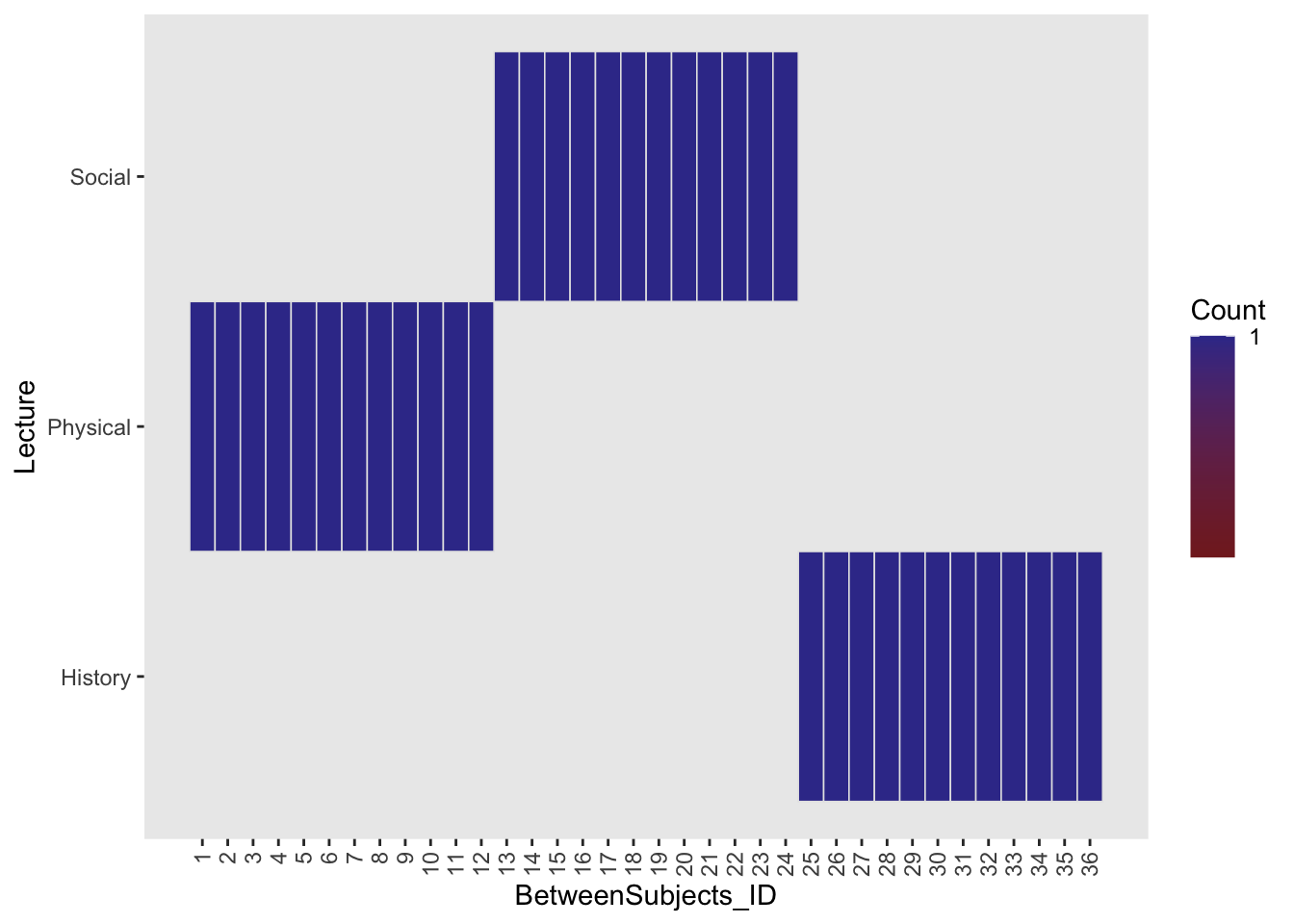
Skipping past the preliminaries (e.g., testing for assumptions) and straight to running the BS ANOVA. Note that I’m using lm() here only to prove a point.
between_aov <- lm(Score~Lecture, data = within_between)
rstatix::anova_test(between_aov, effect.size = "ges")
ANOVA Table (type II tests)
Effect DFn DFd F p p<.05 ges
1 Lecture 2 33 4.284 0.022 * 0.206However, let’s assume instead that this data set was collected using within design. That is, instead of different participants in each Lecture group, the same group of people went through all three lectures:
ez::ezDesign(within_between,y=Lecture,x=WithinSubjects_ID)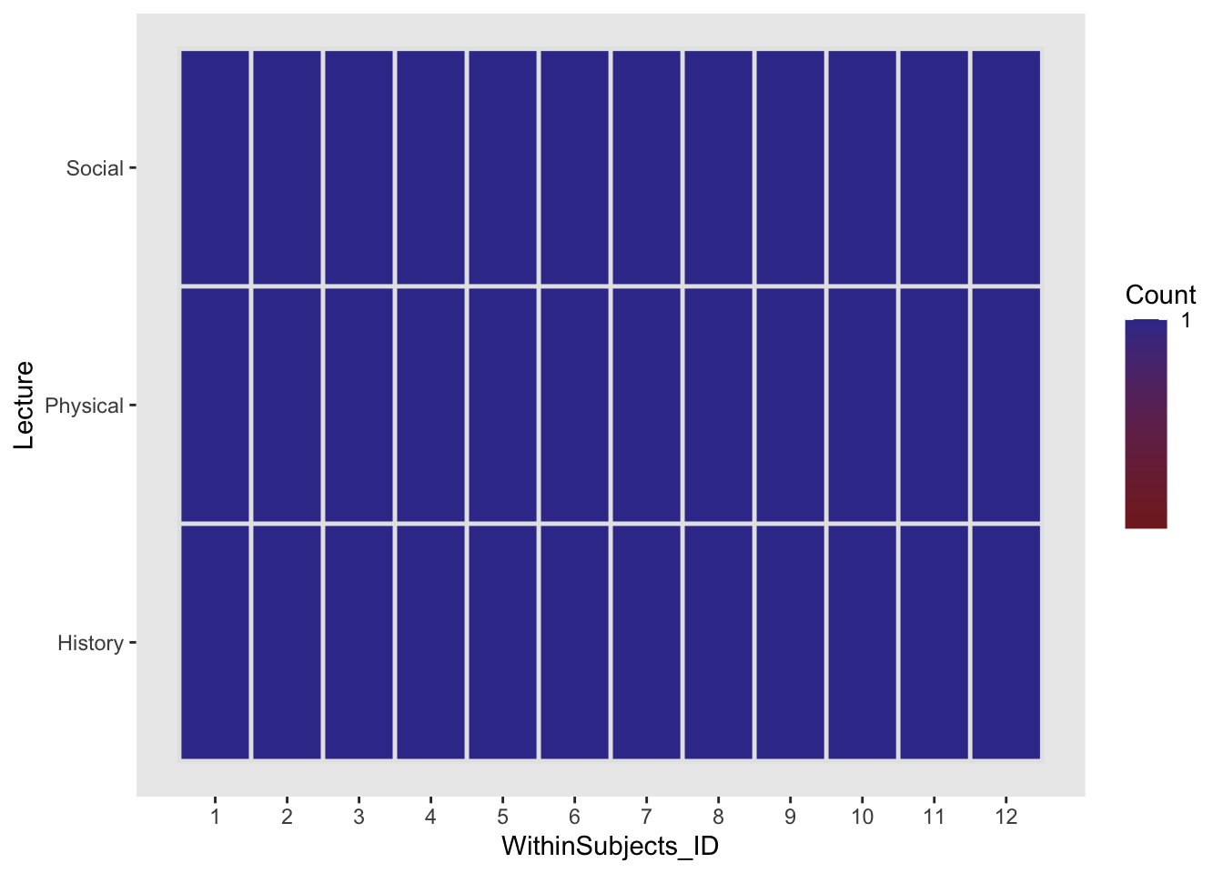
We see that the ezDesign has changed. Instead of 36 participants each individually assigned to a single condition, we have 12 participants each assigned to all three conditions for a single trial (measure). As I briefly mentioned in class, conceptually, a within subjects design considers participant as a pseudo factor with each individual participant as a level. To fully capture this we should factorize our WithinSubjects_ID column.
Running the within-subjects ANOVA:
ANOVA Table (type II tests)

                     Effect DFn DFd      F        p p<.05   pes
1                   Lecture   2  22 12.305 2.59e-04     * 0.528
2 factor(WithinSubjects_ID)  11  22  6.618 8.94e-05     * 0.768
Before continuing on, I want you to take a moment and think about what the specification of the formula in the lm() model above actually means. Not only are we using Lecture as a predictor, but we are also treating participant WithinSubjects_ID as a (psuedo) factor as well. That is not only is the model accounting for the variation moving between levels of Lecture, but also the model is accounting for variability moving between each participant. If you want to continue to use the lm() method for model building, you will need to include participant as a factor in the model. However, I would not recommend continuing with lm(), especially as you end up with more complex within-subjects designs. In your future, you will probably elect to run either a mixed effects model using lmer or a repeated measures ANOVA. Mixed effect modeling is outside of the scope of what we cover this semester (although we’ve laid some foundations for it).
As for repeated measures ANOVA, I would recommend turning to our new friend afex.
46.1.2 Between v. Within ANOVA
Let’s specify a between-subjects ANOVA model using the afex package. I personally prefer the formula method of aov_car()…
# aov_car method
between_aov <- afex::aov_car(Score~Lecture + Error(BetweenSubjects_ID), data = within_between)
Converting to factor: LectureContrasts set to contr.sum for the following variables: Lecturebut in this walkthrough I’ll be using the argument method of aov_ez(). Remember that BOTH do the same thing.
# aov_ez method (alternative)
between_aov <- afex::aov_ez(
  id = "BetweenSubjects_ID",
  dv = "Score",
  data = within_between,
  between = "Lecture")
Converting to factor: LectureContrasts set to contr.sum for the following variables: LectureFrom here we can obtain a look at our ANOVA by calling anova() like so:
anova(between_aov, es = "ges")Anova Table (Type 3 tests)
Response: Score
num Df den Df MSE F ges Pr(>F)
Lecture 2 33 139.36 4.2838 0.20611 0.02218 *
---
Signif. codes: 0 '***' 0.001 '**' 0.01 '*' 0.05 '.' 0.1 ' ' 1Things become a little more complex when we want to run a within-subjects ANOVA. We need to specify the error term in a slightly different way, by acknowledging that the error term is a function of the nesting between our independent variable and our participants (i.e., multiple levels of the IV are nested withing each subject). Using aov_car we specify the error term as Error(WithinSubjects_ID/Lecture).
within_aov <- afex::aov_car(Score~Lecture + Error(WithinSubjects_ID/Lecture), data = within_between)Using aov_ez we simply list the variables under the within argument (well, we also need to change the id column, due to how I’ve constructed the demo set.
# aov_ez method (alternative)
within_aov <- afex::aov_ez(
  id = "WithinSubjects_ID",
  dv = "Score",
  data = within_between,
  within = "Lecture")
We can also get a glimpse of our results using:
anova(within_aov, es = "pes", correction = "none")Anova Table (Type 3 tests)
Response: Score
num Df den Df MSE F pes Pr(>F)
Lecture 2 22 48.515 12.305 0.52801 0.000259 ***
---
Signif. codes: 0 '***' 0.001 '**' 0.01 '*' 0.05 '.' 0.1 ' ' 1You may have noted that in the within case I added the argument correction = "none" to the anova() call. We’ll talk more about that in a bit.
For now, remember that in both of these cases the data is exactly the same. What has changed is how we parse the variance (you’ll notice that the denominator degrees of freedom are different for the second ANOVA). In a within design, we need to take into account the “within-subject” variance. That is how individual subjects vary from one level of treatment to the other. In this respect, within designs are typically more powerful than analogous between designs. While the inherent differences between individual subjects is present in both types of designs, your within-subjects ANOVA model includes it in its analysis. In the present example, this increase in power is reflected by the lower MSE (48.52 v. 139.36) and subsequently, larger F-value (12.31 v. 4.28) and effect size (0.53 v. 0.21) in our within-subjects analysis.
Well if that’s the case why not run within-subject (WS) designs all of the time. Well, typically psychologists do when the subject lends itself to WS-designs. BUT there are certainly times when they are not practical, for example, if you are concerned about learning, practice, or carryover effects where exposure to a treatment on one level might impact the other levels—if you were studying radiation poisoning and had a placebo v. radiation dose condition, it be likely that you wouldn’t run your experiment as a within—or at the very least you wouldn’t give them the radiation first. It would also be likely that you’d be in violation several standards of ethics.
46.2 a note on sphericity for Repeated measures ANOVA
In addition to the assumptions that we are familiar with, repeated-measures ANOVA has the additional assumption of Spherecity of Variance / Co-variance. We talk at length in class re: Spherecity of Variance / Co-variance so I suggest revisiting the slides for our example. At the same time there are debates as to the importance of sphericity in the subjects data. One alternative method that avoids these issues is to invoke mixed models (e.g., lmer). However, if you really want to go down the rabbit hole check out Doug Bates reponse on appropriate dfs and p-values in lmer. You’ll note that these discussions were ten years ago and are still being debated (see here. That said, you may be seeing mixed models in your near future (i.e., next semester)
For now, we won’t go down the rabbit hole and just focus on the practical issues confronted when running a repeated-measures ANOVA.
46.3 EXAMPLE 1
To start, we will use data related to the effectiveness of relaxation therapy to the number of episodes that chronic migraine sufferers reported. Data was collected from each subject over the course of 5 weeks. After week 2 the therapy treatment was implemented effectively dividing the 5 weeks into two phases, Pre (Weeks 1 & 2) and Post (Weeks 3,4, & 5).
46.3.1 loading in the data:
example1 <- read_delim("https://www.uvm.edu/~statdhtx/methods8/DataFiles/Tab14-3.dat", delim = "\t")Rows: 9 Columns: 6
── Column specification ────────────────────────────────────────────────────────
Delimiter: "\t"
dbl (6): Subject, Wk1, Wk2, Wk3, Wk4, Wk5
ℹ Use `spec()` to retrieve the full column specification for this data.
ℹ Specify the column types or set `show_col_types = FALSE` to quiet this message.example1# A tibble: 9 × 6
Subject Wk1 Wk2 Wk3 Wk4 Wk5
<dbl> <dbl> <dbl> <dbl> <dbl> <dbl>
1 1 21 22 8 6 6
2 2 20 19 10 4 4
3 3 17 15 5 4 5
4 4 25 30 13 12 17
5 5 30 27 13 8 6
6 6 19 27 8 7 4
7 7 26 16 5 2 5
8 8 17 18 8 1 5
9 9 26 24 14 8 9You’ll notice that the data set above is in wide format. Each subject is on a single row and each week is in its own column. Note that this is the preferred format for within subjects analysis for SPSS. However in R we want it in long format.
example1_long <- pivot_longer(example1,
                              cols = -Subject,
                              names_to = "Week",
                              values_to = "Migraines")

example1_long$Week <- as.factor(example1_long$Week)
example1_long$Subject <- as.factor(example1_long$Subject)

example1_long
# A tibble: 45 × 3
Subject Week Migraines
<fct> <fct> <dbl>
1 1 Wk1 21
2 1 Wk2 22
3 1 Wk3 8
4 1 Wk4 6
5 1 Wk5 6
6 2 Wk1 20
7 2 Wk2 19
8 2 Wk3 10
9 2 Wk4 4
10 2 Wk5 4
# ℹ 35 more rowsOk, much better, each Subject × Week observation is on a single row.
46.3.2 plotting the data
In addition to plotting your means, one crucial step is to plot the changes in the within-subject (repeated measures) variable at the participant-level. This is especially useful for discerning whether the pattern of results is roughly similar for all participants -OR- if, instead there is large individual variability in the direction of the effect. In other words, “is your manipulation having roughly the same effect for every participant OR is the effect drastically different for participants.
There are 2 ways to do this: 1. the Facet plot or 2. Spaghetti Plot.
46.3.3 the Facet plot
Each window / facet is for a single subject (S1-S9):
ggplot(data = example1_long, aes(x=Week, y=Migraines, group = 1)) +
  geom_point() +
  geom_line() +
  facet_wrap(~Subject, ncol = 3)
46.3.4 the Spaghetti Plot
In this case each line represents an individual Subject (1-9):
ggplot(data = example1_long, aes(x=Week, y=Migraines, group = Subject)) +
  geom_point(aes(col=Subject)) +
  geom_line(aes(col=Subject))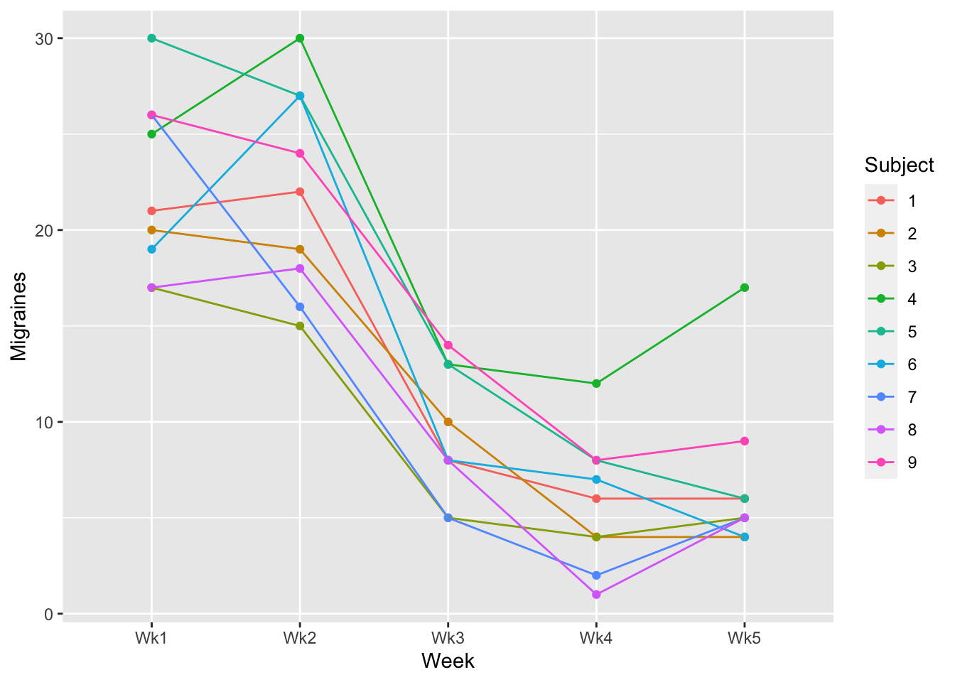
Which you choose is ultimately up to you. I tend to use Spaghetti plots unless I have instances where I have a high number of participants. This can potentially make the spaghetti plot busy (a bunch of points and line). That said, the purpose of the Spaghetti Plot is to note inconsistencies in trends. A helpful tool for an overcrowded Spaghetti Plot is to use plotly. This produces an interactive plot where you can use the mouse cursor to identify important information:
pacman::p_load(plotly) # may need to install

s_plot <- ggplot(data = example1_long, aes(x=Week, y=Migraines, group = Subject)) +
  geom_point(aes(col=Subject)) +
  geom_line(aes(col=Subject))

plotly::ggplotly(s_plot)
Try hovering over individual points and lines in the plot above. Also, see what happens when you click on one of the participant numbers in the legend.
For now this all the plotting we will do. Camera ready summary plots of repeated measures designs add a layer of complexity that warrants its own walkthrough.
46.3.5 building the model using afex:
Running a WS ANOVA is just like running a BS ANOVA in afex (see the last walkthrough). We call in our within subjects factors using the within= argument.
within_aov <- afex::aov_ez(id = "Subject",
                           dv = "Migraines",
                           data = example1_long,
                           between = NULL,
                           within = "Week"
                           )

# alternatively, we can use the formula interface of aov_car

# afex::aov_car(Migraines ~ Week + Error(Subject/Week), data = example1_long)
46.3.6 assumptions checks: normality
We can then use the model, within_aov to run the requisite assumption checks. As before, the model plays nicely with performance, but the blanket check_model will not work with afex. Instead we can do a piecemeal check for normality along with visualizations. For some strange reason, when using afex we need to explicitly print() the output.
within_aov %>% performance::check_normality() %>% print()OK: residuals appear as normally distributed (p = 0.206).46.3.7 assumptions checks: sphericity
Just like the paired \(t\) test from a few weeks back, the RM-ANOVA does not have an explicit check for homogeneity of variance. Instead, RM ANOVA introduces a new test of assumptions that you must run, the Mauchly Tests for Sphericity. Indeed, this test is run instead of the check for homogeneity. This is because technically a WS ANOVA violates the assumption of independence of scores, and thus inflates the likelihood of a homogeneity of variances violation. Essentially, we give up on trying to hold onto the homogeneity assumption (resistance is futile) and instead direct our interests towards maintaining sphericity. Importantly, if we do violate sphericity, there is a clean and relatively agreed upon step that we must take with our analysis.
We can again use the performance library to check for sphericity (you can ignore the warning here):
performance::check_sphericity(within_aov) %>% print()Warning in summary.Anova.mlm(object$Anova, multivariate = FALSE): HF eps > 1
treated as 1OK: Data seems to be spherical (p > 0.537).In this case the results of Mauchly’s test suggest we are ok (in this case \(p > .05\)). Now we can simply grab the output of our ANOVA, specifyingcorrection = "none".
anova(within_aov, es = "pes", correction = "none")Anova Table (Type 3 tests)
Response: Migraines
num Df den Df MSE F pes Pr(>F)
Week 4 32 7.2 85.042 0.91402 < 2.2e-16 ***
---
Signif. codes: 0 '***' 0.001 '**' 0.01 '*' 0.05 '.' 0.1 ' ' 1That being said, there is an argument to be made that you should always make a correction to guard against deviations from sphericity. The correction becomes larger the further your data is from perfect sphericity (which can never truly be obtained in real data). However, standard practice in the psychology literature is to only apply the correction if our data fail the Mauchly’s Test (p < .05) link, so we will proceed on to the next steps.
46.3.8 running post-hoc analyses and follow-ups
Post-hoc comparisons of means take a different form for repeated measures ANOVA. Typical methods such as Tukey HSD were designed for between-subjects effects, where it makes sense (assuming homogeneity of variance) to use a pooled error term. However, mutl
The typical recommendation (more detail on this in the following walkthrough) is to carry out pair-wise contrasts for a within-subjects factor using ordinary paired tests with an error term based only on the levels being compared.
Let’s briefly think back to when we were running post-hoc (and simple effects) analyses on Between Subject ANOVA. A point was made that pairwise comparisons should be considered in light of the full model, meaning that the tests needed to consider the Error terms, including df from the omnibus ANOVA. Simply put, the recommendation above is saying that you should NOT do the same when running a repeated measures ANOVA.
emm_Week <- emmeans(within_aov, specs = ~Week)
emm_Week %>% pairs()
contrast estimate SE df t.ratio p.value
Wk1 - Wk2 0.333 1.700 8 0.196 0.9996
Wk1 - Wk3 13.000 1.247 8 10.423 <.0001
Wk1 - Wk4 16.556 1.375 8 12.036 <.0001
Wk1 - Wk5 15.556 1.608 8 9.672 0.0001
Wk2 - Wk3 12.667 1.179 8 10.748 <.0001
Wk2 - Wk4 16.222 0.909 8 17.837 <.0001
Wk2 - Wk5 15.222 1.441 8 10.562 <.0001
Wk3 - Wk4 3.556 0.818 8 4.345 0.0154
Wk3 - Wk5 2.556 1.156 8 2.211 0.2663
Wk4 - Wk5 -1.000 0.882 8 -1.134 0.7857
P value adjustment: tukey method for comparing a family of 5 estimates Note that the df (df = 8) of these tests are NOT the error df (df = 22) from the omnibus ANOVA. Also note that the SE of each comparison is different.
46.3.9 Example 1 write up
To test whether relaxation therapy had a positive effect for migraine suffers, we analyzed the number of migraines each individual reported over a 5 week period. The first two weeks were used as a baseline to establish a typical week for each person. The remaining three weeks each person was lead through relaxation therapy techniques. These data were submitted to a within-subjects ANOVA with Week as a factor.
Post hoc comparisions demonstrated the effectiveness of our treatment. While the number of migraines remained indifferent during the first two weeks (TukeyHSD, p >.05) there was a significant decrease in the number of migraines post treatment—the number of migraines in Weeks 3, 4, 5 we significantly lower than Weeks 1 and 2 (ps < .05).
** note that you don’t have to worry about the sphericity violation as it relates to the pairwise post hoc analyses—as you are only comparing two levels.
46.4 EXAMPLE 2
Let’s take a look at another example, using a experimental paradigm we are familiar with, scores as a function of lecture type.
46.4.1 loading in the data
You note that this data is already in long format so no need to adjust.
example2_long <- read_csv("http://tehrandav.is/courses/statistics/practice_datasets/withinEx2.csv")Rows: 36 Columns: 3
── Column specification ────────────────────────────────────────────────────────
Delimiter: ","
chr (1): Lecture
dbl (2): Subject, Score
ℹ Use `spec()` to retrieve the full column specification for this data.
ℹ Specify the column types or set `show_col_types = FALSE` to quiet this message.example2_long# A tibble: 36 × 3
Subject Lecture Score
<dbl> <chr> <dbl>
1 1 Physical 53
2 2 Physical 49
3 3 Physical 47
4 4 Physical 42
5 5 Physical 51
6 6 Physical 34
7 7 Physical 44
8 8 Physical 48
9 9 Physical 35
10 10 Physical 18
# ℹ 26 more rows46.4.2 plotting the data
Why don’t you try to create a Spaghetti plot!!!
46.4.3 running the ANOVA:
As before, let’s run this using afex:
within_aov <- afex::aov_ez(
  id = "Subject",
  dv = "Score",
  data = example2_long,
  between = NULL,
  within = "Lecture"
)

# alternative with aov_car:

# within_aov <-
#   afex::aov_car(Score ~ Lecture + Error (Subject/Lecture),
# data = example2_long)performance::check_sphericity(within_aov)Warning: Sphericity violated for:
- (p = 0.012).You’ll notice that in this example the data failed the Mauchly Test for Sphericity (\(p\) = .012). In this case you’ll need to make the appropriate corrections. To do so you have two possibile choices, the Greenhouse-Geisser method or the Huynh-Feldt method.
The Greenhouse-Geisser (GG) correction is more conservative and is generally recommended when the epsilon value from Mauchly’s Test is less than .75. It adjusts the degrees of freedom used in significance testing, thereby increasing the robustness of the results against violations of sphericity.
The Huynh-Feldt (HF) correction is less conservative and may be more appropriate when the epsilon is greater than .75, suggesting a lesser degree of sphericity violation. It also modifies the degrees of freedom but to a lesser extent than GG, resulting in a less stringent correction.
GG corrections are the “industry standard” (you typically see these in psych literature). Let’s go ahead an do this now and return to HF methods at the end of the walk through.
anova(within_aov, es = "pes", correction = "GG")Anova Table (Type 3 tests)
Response: Score
num Df den Df MSE F pes Pr(>F)
Lecture 1.262 13.882 76.885 12.305 0.52801 0.00225 **
---
Signif. codes: 0 '***' 0.001 '**' 0.01 '*' 0.05 '.' 0.1 ' ' 146.4.4 post-hocs and follow-ups
emmeans(within_aov,
        spec= ~Lecture) %>%
  pairs(adjust="tukey")
contrast estimate SE df t.ratio p.value
Physical - Social 14.0 3.01 11 4.651 0.0019
Physical - History 5.5 1.52 11 3.618 0.0104
Social - History -8.5 3.59 11 -2.368 0.0875
P value adjustment: tukey method for comparing a family of 3 estimates 46.4.5 Example 2 write up
Again I need to get my summary stats for the write up. Since I’m not doing any custom contrasts I can just pull the cell values from my summary table:
example2_long %>%
  group_by(Lecture) %>%
  rstatix::get_summary_stats(Score, type ="mean_se")
# A tibble: 3 × 5
Lecture variable n mean se
<chr> <fct> <dbl> <dbl> <dbl>
1 History Score 12 34.5 2.42
2 Physical Score 12 40 3.12
3 Social Score 12 26 4.39And now for the write-up:
… to test this hypothesis we ran a within subjects ANOVA. Due to a violation of the sphericity assumption, we used Greenhouse-Geisser corrected degress of freedom. Our analysis revealed a significant effect for Lecture, \(F\)(1.26, 13.88) = 12.31, \(p\) = .002, \(\eta_p^2\) = .53. Post-hoc analyses revealed participants scores in the Physical condition (\(M\) ± \(SE\): 40.0 ± 3.12) was significantly greater than both History (34.5 ± 2.4) and Social (26.0 ± 4.4) scores (\(p\)s < .05). History and Social were not different from one another.
Take a look at the next walkthrough for an example of factorial repeated measures ANOVA.
46.5 a note on using the Huynh-Feldt correction and how these funky \(df\) are calculated.
As mentioned above, GG corrections are the “standard” and typically show up in psychology literature. However, if one is willing to be less conservate (i.e., accept more risk of Type 1 error) then they may elect to use HF corrections assuming the criteria have been met. Remembner that HF is less conservative and only really appropriate when the epsilon is greater than .75 (i.e., there is a lesser degree of spherecity violation). Unfortunately performance::check_spherecity() doesn’t give us an output of epsilon, only the resulting p_value. Using the model from example 2:
performance::check_sphericity(within_aov) %>% print()Warning: Sphericity violated for:
- (p = 0.012).Fortunately, afex has it’s own baked in test that can be used instead of performance. That said, it involves print out a ton of results
summary(within_aov)
Univariate Type III Repeated-Measures ANOVA Assuming Sphericity

            Sum Sq num Df Error SS den Df F value    Pr(>F)
(Intercept)  40401      1   3531.7     11 125.836 2.319e-07 ***
Lecture       1194      2   1067.3     22  12.305  0.000259 ***
---
Signif. codes:  0 '***' 0.001 '**' 0.01 '*' 0.05 '.' 0.1 ' ' 1


Mauchly Tests for Sphericity

        Test statistic  p-value
Lecture        0.41524 0.012345


Greenhouse-Geisser and Huynh-Feldt Corrections
 for Departure from Sphericity

         GG eps Pr(>F[GG])
Lecture 0.63101    0.00225 **
---
Signif. codes:  0 '***' 0.001 '**' 0.01 '*' 0.05 '.' 0.1 ' ' 1

           HF eps Pr(>F[HF])
Lecture 0.6748954 0.00173583
The output above can be broken down into three parts:
- the top contains the actual output of the ANOVA minus the corrections.
- the second section is the Mauchly test.
- the third part includes the epsilons (eps) for both the GG and HF tests, as well as whether the resulting model is significant.
In this case the HF eps (0.675) is not > 0.75 so we should use the GG correction. If we were doing this by hand, this would involve taking the GG eps, \(\epsilon\) , and multiplying it by our predictors original \(df\) to get the corrected \(df\).
\[ \text{corrected num }df = \text{original numerator } df \; \times \; \epsilon \newline \text{corrected den }df = \text{original denominator } df \; \times \; \epsilon \]
In this case that is 2 * 0.63101 ≈ 1.26 and 22 * 0.63101 ≈ 13.88. You’ll note that these are the \(df\) from:
anova(within_aov, es = "pes", correction = "GG")Anova Table (Type 3 tests)
Response: Score
num Df den Df MSE F pes Pr(>F)
Lecture 1.262 13.882 76.885 12.305 0.52801 0.00225 **
---
Signif. codes: 0 '***' 0.001 '**' 0.01 '*' 0.05 '.' 0.1 ' ' 1If instead we decided we wanted to take more risk and use HF, we would perform the exact sampe process only using HF eps. To impliment this in our anova() we simply change the call to correction = "HF".
anova(within_aov, es = "pes", correction = "HF")Anova Table (Type 3 tests)
Response: Score
num Df den Df MSE F pes Pr(>F)
Lecture 1.3498 14.848 71.885 12.305 0.52801 0.001736 **
---
Signif. codes: 0 '***' 0.001 '**' 0.01 '*' 0.05 '.' 0.1 ' ' 1You notice that the resulting \(df\)s are different.
OK. Let’s move onto the next walkthrough where we look at factorial repeated measures ANOVA.