pacman::p_load(car, # qqPlot function
               cowplot, # apa plotting
               tidyverse, # tidyverse goodness
               psych, # descriptive stats
               lm.beta # getting a standard coefficient
) 22 Correlations
In this week’s readings and lecture we cover correlation and regression. In what follows we will revisit the ideas from this week’s readings and notes, making explicit callbacks to topics from slides and using an example.
Please note that this walkthrough assumes that you have the following packages installed and loaded in R:
22.1 The Relationship b/tw Stress and Health
Wagner, Compas, and Howell (1988) investigated the relationship between stress and mental health in first-year college students. Using a scale they developed to measure the frequency, perceived importance, and desirability of recent life events, they created a measure of negative events weighted by the reported frequency and the respondent’s subjective estimate of the impact of each event. This served as their measure of the subject’s perceived social and environmental stress. They also asked students to complete the Hopkins Symptom Checklist, assessing the presence or absence of 57 psychological symptoms.
This data can be accessed directly from this companion website for Howell’s stats textbook (a book I used a while back).
stress_data <- read_table("https://www.uvm.edu/~statdhtx/methods8/DataFiles/Tab9-2.dat")
── Column specification ────────────────────────────────────────────────────────
cols(
  ID = col_double(),
  Stress = col_double(),
  Symptoms = col_double(),
  lnSymptoms = col_double()
)psych::describe(stress_data) vars n mean sd median trimmed mad min max range skew
ID 1 107 54.00 31.03 54.00 54.00 40.03 1.00 107.00 106.00 0.00
Stress 2 107 21.29 12.49 20.00 20.49 11.86 1.00 58.00 57.00 0.62
Symptoms 3 107 90.33 18.81 88.00 88.87 17.79 58.00 147.00 89.00 0.74
lnSymptoms 4 107 4.48 0.20 4.48 4.48 0.19 4.06 4.99 0.93 0.21
kurtosis se
ID -1.23 3.00
Stress -0.19 1.21
Symptoms 0.45 1.82
lnSymptoms -0.28 0.0222.1.1 Testing our assumptions
Here we are interested in the relationship between perceived Stress (as measured on a scale factors the number and impact of negative life events) and the presence of psychological Symptoms. As with any other parametric analysis, we first need to see if our data adheres to the assumption of normality. We can use the tools we learned in Part 5 to test this assumption.
Let’s call in the performance package to perform some visual inspection.
First Stress.
Step 1: Quick Shapiro Wilkes
As a first pass we might check using the Shapiro-Wilkes test. The Shapiro-Wilkes test (\(W\)) of normality compares our observed distribution against a theoretical normal. Here the null hypothesis is that the \(observed == theoretical\), where \(p < .05\) indicates that the observed distribution is not normal. In Field’s text he showed you the shapiro.test() function:
shapiro.test(stress_data$Stress) # see Field (2014), Sec 5.6.1
    Shapiro-Wilk normality test

data:  stress_data$Stress
W = 0.96009, p-value = 0.002709
I recommend using the performance::check_normality() function. In order to apply this function to raw data we’ll need create an intercept only model with our data:
intercept_only_stress_mdl <- lm(formula = Stress~1,
                                data = stress_data)
performance::check_normality(intercept_only_stress_mdl)
Warning: Non-normality of residuals detected (p = 0.003).If you look at the ?help for performance::check_normality you’ll note that it actually invokes shapiro.test. I simply prefer it for the sake of being consistant as I use performance as a one-stop-shop for all my assumption checking (well most of it anyway). That said, one thing you may have noted is that performance::check_normality() doesn’t give you the \(W\) statistic. In the rare event that you are asked, or want to report this then you’ll have to get it from shapiro.test().
Either way, our obtained \(p-value\) suggests the possibility that Stress measures deviate from normal. However, as noted in the Field text we need to be careful using the Shapiro-Wilkes test on large samples.
With this in mind I would move on to the next step, visualization.
Step 2: Visualization
What’s nice about using performance is that I can take the same call that I used to invoke Shapiro-Wilkes and pipe it to a plotting function to generate a qq-plot:
performance::check_normality(intercept_only_stress_mdl) %>%
  plot("qq")
Eyeballing the plots, our Stress measures look slightly skewed, but not egregiously so. For instance, only one of the data points falls outside the 95% CI band (shaded area). If I get a conflict between Step 1 and Step 2, then I’d move on to the next step.
Step 3: Quantifying Skew and Kurtosis
Let’s take a look at the skew and kurtosis values. Refering to Walkthrough 19 you’ll note that I recommend the method using bootstrapped standard errors. This entails dividing our skew value (from psych::describe or psych::skew by the standard error of the skew. Recall, to get the standard error of the skew, the best way is to bootstrap a sampling distribution.
First let’s get the sample skew:
psych::skew(stress_data$Stress)[1] 0.61812Here I’m just going to bootstrap the skew using DescTools::Skew() and get the 95% CI
boot_skew_data <- DescTools::Skew(stress_data$Stress, method = 2, ci.type = "bca",conf.level = .95)Then to get the standard error I can just divide the range of the ci by 3.92 (95% of a normal distribution falls withing ±1.96 SD of the mean; the standard error = 1 SD).
standard_error_skew <- (boot_skew_data["upr.ci"] - boot_skew_data["lwr.ci"])/3.92
standard_error_skew
upr.ci
0.1787086 Now we can divide our the skew of the actual sample (0.62) by the standard_error_skew (0.19) and evaluate the result against the criteria mentioned in class. (Again if we are being diligent we would repeat this for kurtosis).
.62 / .19[1] 3.263158That said, recall from Part 5 that we created a custom function to do all of this for us. Let’s source it:
source("http://tehrandav.is/courses/statistics/custom_functions/skew_kurtosis_z.R")And use it:
skew_kurtosis_z(stress_data$Stress) upr.ci crit_vals
skew_z 3.18 3.29
kurt_z -0.36 3.29Using the criteria set forth in Kim (2013), this data is indeed skewed (> 3.29). Given our obtained score is greater than the critical value (\(3.35 > 3.29\)) this method suggests that the data is indeed non-normal.
Now Symptoms
I’m just going to do this all in one-fell-swoop:
intercept_only_symptoms_mdl <- lm(Symptoms ~ 1, stress_data)
performance::check_normality(intercept_only_symptoms_mdl)
Warning: Non-normality of residuals detected (p = 0.002).performance::check_normality(intercept_only_symptoms_mdl) %>% plot("qq")
skew_kurtosis_z(stress_data$Symptoms) upr.ci crit_vals
skew_z 3.68 3.29
kurt_z 0.77 3.29Symptoms does not pass any of our checks.
One way of dealing with non-normal data is by performing a logarithmic transformation (see Field, 5.8). Logarithmic transformations reduce the weight of extreme scores. For example, consider the following vector:
c(2,4,6,8,100)[1] 2 4 6 8 100100 is setting way out to the extreme of the other scores. Now let’s get the log() of this sequence:
c(2,4,6,8,100) %>% log()[1] 0.6931472 1.3862944 1.7917595 2.0794415 4.6051702The values become more manageable (i.e., closer) at this rescaling.
This has already been performed for this data, lnSymptoms is a natural logarithmic transform of Symptoms. With your own data, this can be accomplished quite simply in R by using the log() as above. Let’s apply a log transform to our Stress data.
stress_data <-
  stress_data %>%
  mutate(lnStress = log(Stress))
Now let’s check our assumptions again on both of the log transformed data. For brevity I’m just going to use the bootstrapped ses method.
First, lnSymptoms
skew_kurtosis_z(stress_data$lnSymptoms) upr.ci crit_vals
skew_z 1.27 3.29
kurt_z -0.95 3.29Awesome! Now lnStress:
skew_kurtosis_z(stress_data$lnStress) upr.ci crit_vals
skew_z -4.9 3.29
kurt_z 1.9 3.29Uh-oh, log-transforming Stress doesn’t look like it solved our problem. A visual inspection confirms this:
intercept_only_ln_stress_mdl <- lm(lnStress ~ 1, stress_data)
performance::check_normality(intercept_only_ln_stress_mdl) %>% plot("qq")
In this case it’s probably best to proceed with the log transformed Symptoms lnSymptoms but keep our raw Stress scores.
22.2 Plotting the data
One of the first things that you should do is plot your data. Plotting gives you a sense of what is going on with your data. In fact, YOU SHOULD NEVER TAKE A TEST RESULT AT FACE VALUE WITHOUT FIRST LOOKING AT YOUR DATA!! Beware of Anscombe’s quartet!
To really drive this home, let’s look at an example from a function that Jan Vanhove developed as a teaching tool. the function plot_r() takes an input correlation coefficient r and number of observations n and plots 16 very distrinct types of patterns that can be produced. For the sake of not slowing down your machine too much, I’d recommend keeping n at less than 200.
source("http://janhove.github.io/RCode/plot_r.R")
plot_r(r = 0.5, n = 50)
For what its worth, # 14 is a particulary nasty case that can be addressed by Multi-level modeling (see Field Chapter 19). MLM is outside the scope of this course, but you may encounter it next semester.
For now, let’s plot our data using ggplot. In this case we will be creating a scatterplot of our data. This can be accomplished by adding geom_point() to our base ggplot(). For example:
ggplot(stress_data, aes(x = Stress, y = lnSymptoms)) +
  geom_point() +
  theme_cowplot() + # turns the plot into something close to APA
  xlab("Stress") +
  ylab("lnSymptoms")
22.3 Covariance and Correlation
This week’s readings offer excellent overviews of covariance and correlation so I won’t go into too much depth here. Briefly, let’s make a few connections to ideas that we’ve already encountered.
22.3.1 Covariance
Recall that variance may be calculated as: \[ s_{x}^{2}=\frac{\sum \left ( x_{i}-\bar{X} \right )^{2}}{n-1} \]
Where the numerator is the sum of squared differences from each score to the sample mean, and the denominator is our degrees of freedom.
Variance tells us to what degree scores in a particular sample variable deviate from its mean. With this in mind, covarience is a statement about the degree to which two sampled variables deviate from their respective means. Consider we have sampled two measures, X & Y from a population. When addressing the degree to which X and Y co-vary, we are asking the question: “To what degree and in what direction does Y move away from its mean as X moves from its mean?”
As such, the formula for covariance is simply an extension of the formula for variance that we already know: \[s_{xy}=\frac{\sum \left ( x_{i}-\bar{X} \right )\left ( y_{i}-\bar{Y} \right )}{n-1} \]
So, in order to calculate the covariance we need the calculate the sum of the cross-product of the sum of squared differences of our two variables (X = Stress; Y = lnSymptoms) and divide that number by of degrees of freedom. We could go about the business of calculating this “by hand”:
# N = number of rows in data frame
N <- nrow(stress_data)


#mean Stress:
meanX <- mean(stress_data$Stress)

# and same for lnSymptoms:
meanY <- mean(stress_data$lnSymptoms)

# plug these values into our equation:

# sum of cross product
numerator <- sum((stress_data$Stress-meanX)*(stress_data$lnSymptoms-meanY))

# degrees of freedom
denominator <- (N-1)

# covariance:
covXY <- (numerator/denominator) %>% print()
[1] 1.336434The covariance of Stress and lnSymptoms is 1.336.
Alternatively, covariance may be calculated quickly in R using the cov() function: Remember, once you open up a function, you can press the TAB key to get prompts about what to put in each argument.
cov(stress_data$Stress, stress_data$lnSymptoms)[1] 1.33643422.3.2 Correlation
It may be tempting to calculate our covariance and stop there, but covariance is a limited measure. What I mean by this is that covarience indexes the degree of relationship between two specific variables, but doesn’t allow for more general comparison across situations. For a quick example, lets multiply both Stress and lnSymptoms by two. Let’s use mutate() to create a these by2 columns:
stress_data <- stress_data %>% mutate("Stress_by2" = Stress * 2,
                                    "lnSymptoms_by2" = lnSymptoms * 2
                                    )
stress_data
# A tibble: 107 × 7
ID Stress Symptoms lnSymptoms lnStress Stress_by2 lnSymptoms_by2
<dbl> <dbl> <dbl> <dbl> <dbl> <dbl> <dbl>
1 1 30 99 4.60 3.40 60 9.19
2 2 27 94 4.54 3.30 54 9.09
3 3 9 80 4.38 2.20 18 8.76
4 4 20 70 4.25 3.00 40 8.50
5 5 3 100 4.61 1.10 6 9.21
6 6 15 109 4.69 2.71 30 9.38
7 7 5 62 4.13 1.61 10 8.25
8 8 10 81 4.39 2.30 20 8.79
9 9 23 74 4.30 3.14 46 8.61
10 10 34 121 4.80 3.53 68 9.59
# ℹ 97 more rowsWe would like to think that multiplying every value by a constant should have no effect on our general interpretation of the relationships in our data as the overall relationship in our data remain the same. To help make this apparent, let’s imagine that I weigh 200 lbs (yea… imagine) and my wife weighs 100 lbs. So I weigh twice as much as my wife. Over the next year we both go on a binge fest and both double our respective weights—I’m now 400 lbs and my wife is 200 lbs. I still weigh twice as much as my wife. Coincidentally the fact that relationships remains unchanged in spite of these sorts of mathematical transformations is why we could perform the natural logarithmic transform earlier and not feel too guilty.
Well what happens when I get the covariance of my new _by2 data?:
cov(stress_data$Stress_by2, stress_data$lnSymptoms_by2)[1] 5.345735The covariance changes!! This is a problem, and is why, in order to usefully convey this data we report the correlation. The correlation is a standardized covariance.
The unit of measurement we’ll use for standardization is the standard deviation. We can standardize the covariance in one of two ways:
- Standardize our variables (into z-scores) and then calculate the covariance: \[r_{xy}=\frac{\sum z_{x}z_{y}}{n-1}\]
zX <- scale(stress_data$Stress)
zY <- scale(stress_data$lnSymptoms)

corXY <- (sum(zX*zY) / (N-1))

corXY
[1] 0.5286565or
- Calculate the covariance and standardize it (by dividing by the product of the standard deviation):
- \[r_{xy}=\frac{\sum \left ( x_{i}-\bar{X} \right )\left ( y_{i}-\bar{Y} \right )}{(n-1)s_{x}s_{y}} \]
# get SD of X and Y:
sdX <- sd(stress_data$Stress)
sdY <- sd(stress_data$lnSymptoms)

# using the covXY calculated above:
covXY / (sdX*sdY)
[1] 0.5286565Again, in R we don’t need to do this by hand, there are in fact several functions. A more comprehensive look can be found in Field 6.5.3. The simplest function is cor(), with outputs the correlation as a single value. However, I prefer to use cor.test() as it tends to provide the most immediately useful data. You can input your data into this function in two ways:
cor.test(stress_data$Stress,stress_data$lnSymptoms)or
cor.test(~Stress+lnSymptoms,data = stress_data)
    Pearson's product-moment correlation

data:  Stress and lnSymptoms
t = 6.3818, df = 105, p-value = 4.827e-09
alternative hypothesis: true correlation is not equal to 0
95 percent confidence interval:
 0.3765970 0.6529758
sample estimates:
      cor
0.5286565
I prefer the latter as it uses formula notation which is the sort of notation we used for t-tests and will continue to use for regression and ANOVA.
Our correlation is expressed in terms of the Pearson’s product-moment correlation coefficient (or \(r\), for short). Here \(r\) = .529.
On your own, rerun the cor.test (no need to get the attributes this time) using the problematic by_2 columns. What do you find relative to the last test?
22.4 Adjusted Pearsons’s \(r\)
Note that when our sample size is small (N<30) we may need to adjust \(r\). This is because the sampling distribution of \(r\) is not normally distributed, most especially when you have strong correlations. Don’t believe me? Let’s bootstap 1000 simulations, this time assuming a sample size of only 20 people.
r_distribution <- tibble(simulation = 1:1000) %>%
  group_by(simulation) %>%
  mutate(r_value = cor.test(~Symptoms+Stress,
                            data = sample_n(stress_data,size = 20, replace = T))$estimate)

# note that $estimate allows me to pull the value out directlyggplot(r_distribution, aes(x = r_value)) +
geom_histogram(bins = 30,
fill = "lightblue",
col = "black") +
theme_cowplot()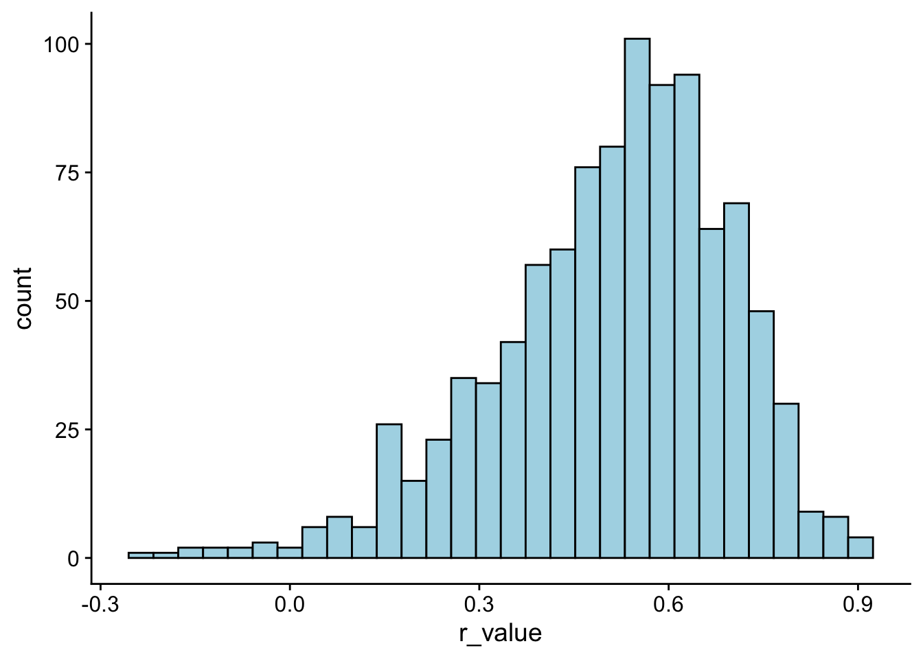
Now, let’s try re-running the above code, this time with sample sizes of 100 instead of 20. What do you see?
# rerun the simulation
r_distribution <- tibble(simulation = 1:1000) %>%
group_by(simulation) %>%
mutate(r_value = cor.test(~Symptoms+Stress,
data = sample_n(stress_data,size = 100, replace = T))$estimate)
ggplot(r_distribution, aes(x = r_value)) +
  geom_histogram(bins = 30,
                 fill = "lightblue",
                 col = "black") +
  theme_cowplot()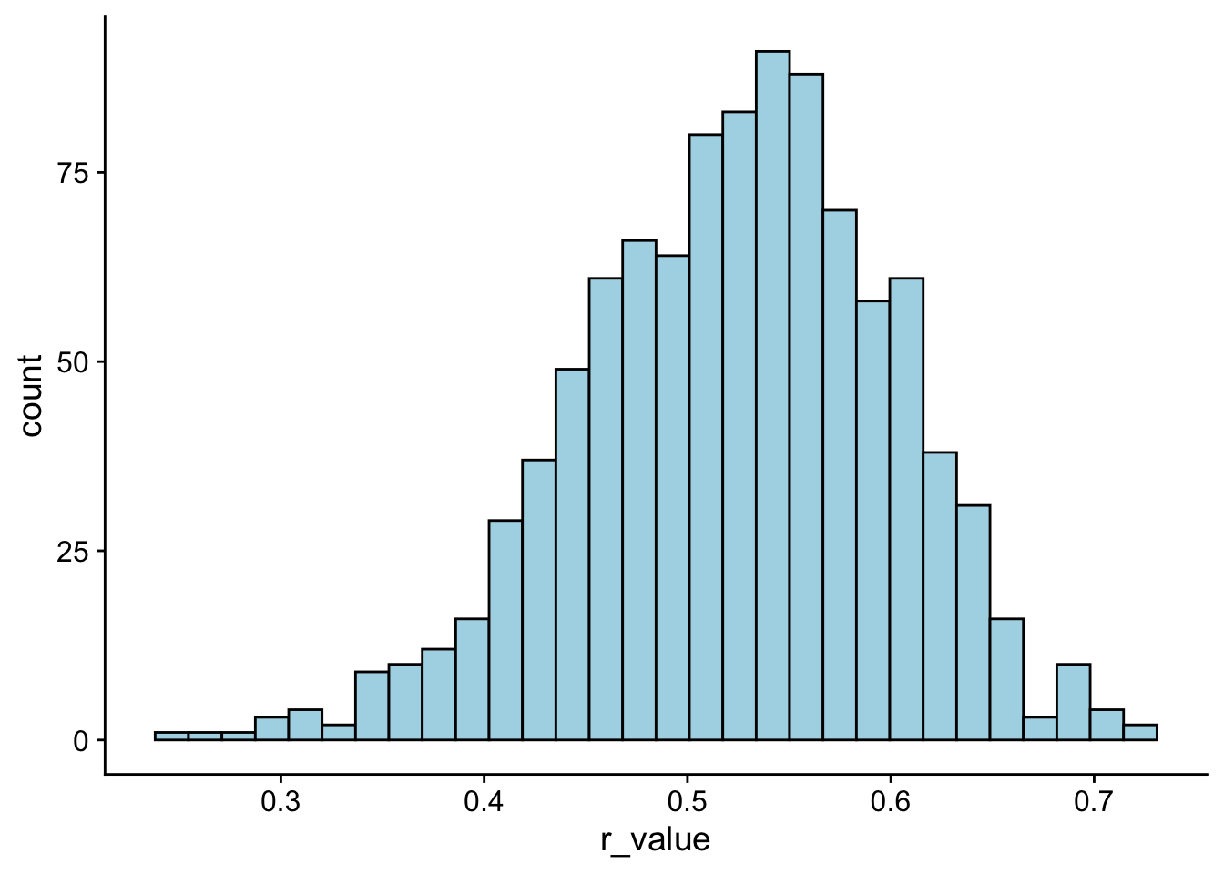
The formula for this adjustment is: \[ r_{adj}=\sqrt{1-\frac{\sum \left (1-r^2 \right )\left ( n-1 \right )}{n-2}} \]
For now, we can calculate this by hand, but later we will see that it will be provided by another function (or at least its squared value will be).
# Pearson's r:
rXY <- cor.test(~Stress+lnSymptoms,data = stress_data)$estimate

# adjusted r:
rXYadj <- sqrt(1-((1-rXY^2)*(N-1)/(N-2))) %>% print()
cor
0.522126 22.5 Significance testing \(r\)
It may be useful to perform tests of significance on \(r\). Typically, there are two types of tests that we perform:
- a test of the observed \(r\) to \(r=0\), and
- a test of the difference between two \(r\) values.
Regarding the first case, to test that the observed correlation is different from 0 we can use the aforementioned cor.test():
cor.test(~Stress+lnSymptoms,data = stress_data)
    Pearson's product-moment correlation

data:  Stress and lnSymptoms
t = 6.3818, df = 105, p-value = 4.827e-09
alternative hypothesis: true correlation is not equal to 0
95 percent confidence interval:
 0.3765970 0.6529758
sample estimates:
      cor
0.5286565
In the second case, the difference between \(r\) values, we may invoke the paired.r() function from the psych package. For example lets assume that we know that the correlation between GRE scores and GPA for one group of 100 students is 0.50 and for another group of 80 students it’s 0.61. We ask is the correlation for the second group significantly higher than the first. To test the difference between these two independent \(r\)s” we
psych::paired.r(xy = .50, n = 100, xz = .61, n2 = 80,twotailed = T)Call: psych::paired.r(xy = 0.5, xz = 0.61, n = 100, n2 = 80, twotailed = T)
[1] "test of difference between two independent correlations"
z = 1.05 With probability = 0.3where:
xy: the correlation in the first data setxz: the correlation in the second data setn: the number of samples in the first data setn2: the number of samples in the second data set -twotailed: run a two-tailed test,TRUEorFALSE
This output tells us the resulting Fisher \(z\) score and corresponding probability.
**Try on your own: Assume that you sample 200 UC undergrads and find a correlation of .29 between Symptoms and Stress. In another sample of 100 graduate students you find a correlation of .51. Perform a test to see if those two correlations are different from one another.
psych::paired.r(xy = .29, n = 200, xz = .51, n2 = 100,twotailed = T)Call: psych::paired.r(xy = 0.29, xz = 0.51, n = 200, n2 = 100, twotailed = T)
[1] "test of difference between two independent correlations"
z = 2.13 With probability = 0.03FWIW… here are my results. Check them against yours.
Call: psych::paired.r(xy = 0.29, xz = 0.51, n = 200, n2 = 100, twotailed = T)
[1] "test of difference between two independent correlations"
z = 2.13  With probability =  0.03