In the example from the previous walkthrough, we collected data from two seperate groups. Because of the design, we felt comfortable that the data from the two samples were independent, at least with respect to any dimensions that might be important to consider. But, what of cases where we knownly violate independence? For example, what if we were to collect data from the same group of people at two different points in time? In this case, we would have two samples that are not independent, but are instead paired. In this case, we would need to run a paired samples\(t\)-test.
When I was a young Assistant Professor a more statistically savvy (and dare I say snobby) colleaguge once remarked to me that “there is no such thing as a ‘repeated samples ANOVA’ test, but only a regular ANOVA were we have violated the independence assumption and are attempting to correct for it.” At this point on my career it was laughable that I would ever be teaching a stats course (I was not strong with the stats as a grad student) and was not entire sure the point my colleague was trying to make, other than perhaps needling me for my data analysis plan.
But, the point is valid… and though made explicilty for ANOVA also applies (and is easier to comprhend) for \(t\) tests. To see whats going on, let’s look at the equation for calculating the \(t\)-statistic assuming an independent samples test:
\[
t = \frac{\bar{X}_1 - \bar{X}_2}{\sqrt{\frac{S^2_1}{n_1} + \frac{S^2_2}{n_2}}}
\]
Essentially we are taking difference between the means of each group \(\bar{X}_1\) and \(\bar{X}X_2\) and dividing that number by the square root of their standard deviations (actually the math in the denominator isn’t quite this, but for our expanation this will do).
Now let’s turn to the equation for the paired samples \(t\)-test:
\[
t = \frac{\bar{D}}{\frac{S_D}{\sqrt{n}}}
\]
In this case, \(\bar{D}\) reflects the mean difference between the two condition, and \(\frac{S_D}\) is the standard deviation of the differences in the paired observations.
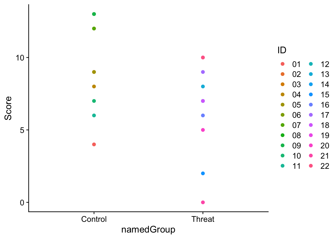
Let’s assume the set of scores from our previous example of sterotype threat. Here’s a plot of each of the data points obtained from the two groups of 11 participants each:
Rows: 22 Columns: 4
── Column specification ────────────────────────────────────────────────────────
Delimiter: ","
chr (2): ID, wID
dbl (2): Score, Group

ℹ Use `spec()` to retrieve the full column specification for this data.
ℹ Specify the column types or set `show_col_types = FALSE` to quiet this message.
ggplot(stereotype_data, aes(x = namedGroup, y = Score, col = ID)) +geom_point(size =2) +theme_cowplot()
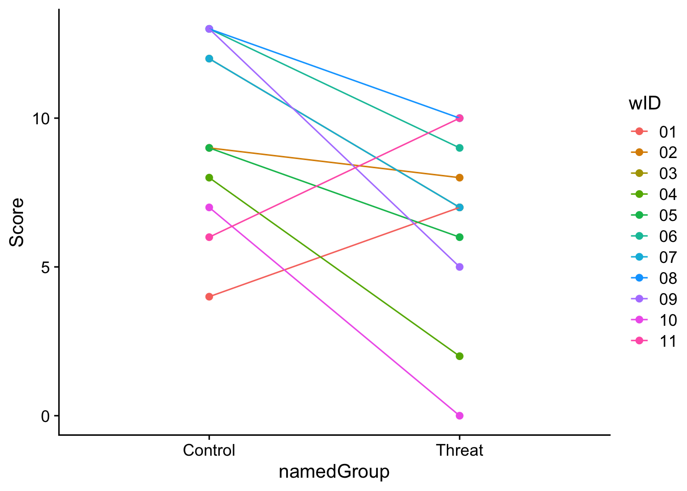
In the case above, we had no we had no basis to believe that a specific data point from one group had a stronger relationship to any particular data point in the other group than to any other data point. That is there was nothing special linking data points between the two groups. Now imagine that instead of two seperate groups, we collected this data from one group of 11 people both in a control condition and under a condition where they were under threat. In this case we might plot the data to include a line connecting the Control and Threat data points for each participant.
ggplot(stereotype_data, aes(x = namedGroup, y = Score, col = wID, group = wID)) +geom_point(size =2) +geom_line() +theme_cowplot()
In this case, we aren’t interested in the individual data points per se but rather how much each individual has changed. To do this, we’ve attached each score to it’s corresponding mate, acknowleding that the scores are related to one another.
For what it’s worth, it is safe to assume that anytime that you are collecting data samples from the same person at two different points in time that you need to run a paired-samples test. However, it would not be safe to assume that if the samples are coming from different groups of people that you always run an independent samples test. Remember the important qualifier mentioned above: That there no reason to believe that any one participant in the first group is is more closely related to any single counterpart in the second group than the remaining of others. In our Independent test example we have no reason to assume this is the case, we assume that members of the Control and Threat groups were randomly selected. But what if we instead recruited brothers or twins? In this case, it may make sense to treat members of the two groups as paired; brothers have a shared history (education, socio-economic level, family dynamic, etc) that would make their scores more likely to be related to one another than by random chance. All of these are scenarios where independence is violated and we need to take into consideration the relationship between scores.
In this walkthrough, we address how this is accomplished in R
27.2 Things to consider before running the t-test
The things to consider in this case are the same as with the independent samples assumption: what is the nature of the data, what is the structure of the data file, and finally running our assumption checks. Let’s grab some sample data and walkthrough each of these as they may come up in a paired samples test.
Hand, et al., 1994, reported on family therapy as a treatment for anorexia. There were 17 teens in this experiment, and they were weighed before and after treatment. The weights of the teens, in pounds, is provided in the data below:
Rows: 17 Columns: 3
── Column specification ────────────────────────────────────────────────────────
Delimiter: ","
chr (1): ID
dbl (2): Before, After

ℹ Use `spec()` to retrieve the full column specification for this data.
ℹ Specify the column types or set `show_col_types = FALSE` to quiet this message.
27.2.1 What is the nature of this data?
So what is known: we have 17 total participants from (hypothetically) the same population that are measured twice (once Before treatment, and once After treatment). Based upon the experimental question we need to run a paired-sample (matched-sample) test. (Although I’ll use this data to provide an example of a one-sample test later on). F
27.2.2 What is the structure of your data file?
Before doing anything you should always take a look at your data:
Most important for present purposes this data is in WIDE format—each line represents a participant. While this might be intuitive for tabluar visualization, many statistical softwares prefer when LONG format, where each line represents a single observation (or some mixed of WIDE and LONG like SPSS).
I spoke a little bit about this issue in Walkthrough 8.
27.2.3 Getting data from WIDE to LONG
So the data are in WIDE format, each line has multiple observations of data that are being compared. Here both Before scores and After scores are on the same line. In order to make life easier for analysis and plotting in ggplot, we need to get the data into LONG format (Before scores and After scores are on different lines). This can be done using the pivot_longer() function from the tidyr package.
Before gathering, one thing to consider is whether or not you have a column that defines each subject. In this case we have ID. This tells R that these data are coming from the same subject and will allow R to connect these data when performing analysis. That said, for t.test() this is not crucially important—t.test() assumes that the order of lines represents the order of subjects, e.g., the first Before line is matched to the first After line. Later on when we are doing ANOVA, however, this participant column will be important an we will need to add if it is missing.
Using pivot_longer(): This function takes a number of arguments, but for us right now, the most important are data: your dataframe; cols: which columns to gather; names_to: what do you want the header of the collaped nonminal variables to be? Here, we might ask what title would encapsulate both Before and After. I’ll choose treatment ; values_to: what do the values represent, here I choose weight. I’m just going to overwrite the original data frame:
# A tibble: 34 × 3
   ID    treatment weight
   <chr> <chr>      <dbl>
 1 01    Before      83.8
 2 01    After       95.2
 3 02    Before      83.3
 4 02    After       94.3
 5 03    Before      86
 6 03    After       91.5
 7 04    Before      82.5
 8 04    After       91.9
 9 05    Before      86.7
10 05    After      100.
# ℹ 24 more rows
Ok data is structured correctly, on to the next step.
27.3 Testing the normality assumption
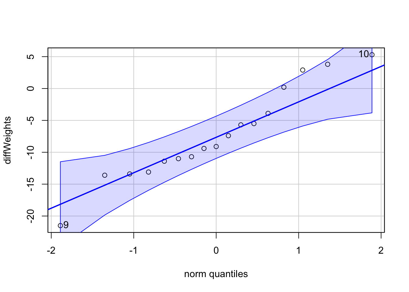
Knowing the design of your experiment also has implications for testing your assumptions. For example, whether you have a paired (matched) sample design (e.g., two samples from the same participants) or an independent sample design (e.g., two seperate groups of people) determines how you go about the business of testing the normality assumption. As we saw in the last walkthrough, if you have an independent samples test, you test each sample separately, noting measures of skew, kurtosis, inspecting the qqPlot, and Shapiro-Wilkes test (though acknowledging that SW is very sensitive). However, if you are running a paired (matched) samples test, you need to be concerned with the distribution of the difference scores. In the present example we are comparing participants’ weights Before treatment to their weight After. This is a paired design, so I need to test the differences between each participant’s Before and After for normality.
First, let me filter() my data accordingly for Before and After (essentially creating separate data frames for each condition):
    Shapiro-Wilk normality test

data:  diffWeights
W = 0.9528, p-value = 0.5023
What conclusions might we draw about normality?
27.4 Homogeneity of variances
With a paired samples test, we do not need to run a check for homogeniety of variance. Let’s think about this. I mentioned above that for a paired-samples test, we are not concerned with the distributions of the two seperate conditions Before and After, but are instead concerned with the distribution of difference scores (Participant 1, Before v. Participant 1, After, etc.). Essentially, we’ve taken those two distributions and reduced them down to a single distribution of scores. There is no need or way to test for the homogeneity of variance assumption when you only have one distribution—the variance is homogenoues to what? itself?
27.5 Getting the descriptive stats
Finally, as we will be performing a test of difference in means, it would be a good idea to get descriptive measures of means and variability for each group. We can use psych::describeBy() to get the means, sds, and ses of each sample.
 Descriptive statistics by group
group: After
   vars  n  mean   sd median trimmed  mad  min   max range  skew kurtosis   se
X1    1 17 90.49 8.49   92.6   90.77 3.85 75.2 101.6  26.4 -0.74    -0.93 2.06
------------------------------------------------------------
group: Before
   vars  n  mean   sd median trimmed  mad  min  max range skew kurtosis   se
X1    1 17 83.23 5.02   83.3   83.15 4.15 73.4 94.2  20.8 0.15    -0.29 1.22
Or, if you prefer you can use some of the skills you got from the DataCamp assignments to generate a more consise table:
# A tibble: 2 × 4
  treatment  mean    sd    se
  <chr>     <dbl> <dbl> <dbl>
1 After      90.5  8.49  2.06
2 Before     83.2  5.02  1.22
Typically along with the mean, you need to report a measure of variability of your sample. This can be either the SD, SE, or if you choose the 95% CI, although this is more rare in the actual report. See the supplied HW example and APA examples for conventions on how to report these in your results section.
27.6 Plotting in ggplot
I’ve mentioned the limits and issues with plotting bar plots, but they remain a standard, so we will simply proceed using these plots. But I’ll note that boxplots, violin plots, bean plots, and pirate plots are all modern alternatives to bar plots and are easy to execute in ggplot(). Try a Google search.
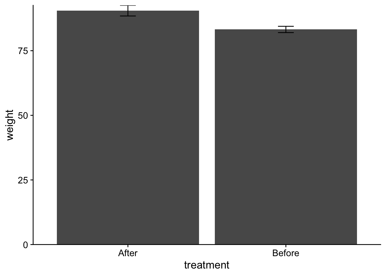
In the meantime, to produce a bar plot in R we simply modify a few of the arguments that we are familiar width.
ggplot(data = anorexia_data, aes(x=treatment, y=weight)): standard fare for starting a ggplot.
stat_summary(fun = "mean", geom = "col"): stat_summary() gets summary statistics and projects them onto the geom of your choice. In this case we are getting the mean values, fun = "mean" and using them to create a column plot geom = "col" .
stat_summary(fun.data = "mean_se", geom = "errorbar", width = .1) : here we are creating error bars, geom = "errorbar". Important to note here is that error bars require knowing three values: mean, upper limit, and lower limit. Whenever you are asking for a single value, like a mean, you use fun. When multiple values are needed you use fun.data. Here fun.data = "mean_se" requests Standard error bars. Other alternatives include 95% CI "mean_cl_normal" and Standard deviation "mean_sdl". The width argument adjusts the width of the error bars.
scale_y_continuous(expand = c(0,0)): Typically R will do this strange thing where it places a gap bewteen the data and the x-axis. This line is a hack to remove this default. It says along the y-axis add 0 expansion (or gap).
theme_cowplot(): quick APA aesthetics.
You may also feel that the zooming factor is off. This may especially be true in cases where there is little visual discrepency between the bars. To “zoom in” on the data you can use coord_cartesian(). For example, you might want to only show the range between 70 lbs and 100 lbs. When doing this, be careful not to truncate the upper limits of your bars and importantly your error bars.
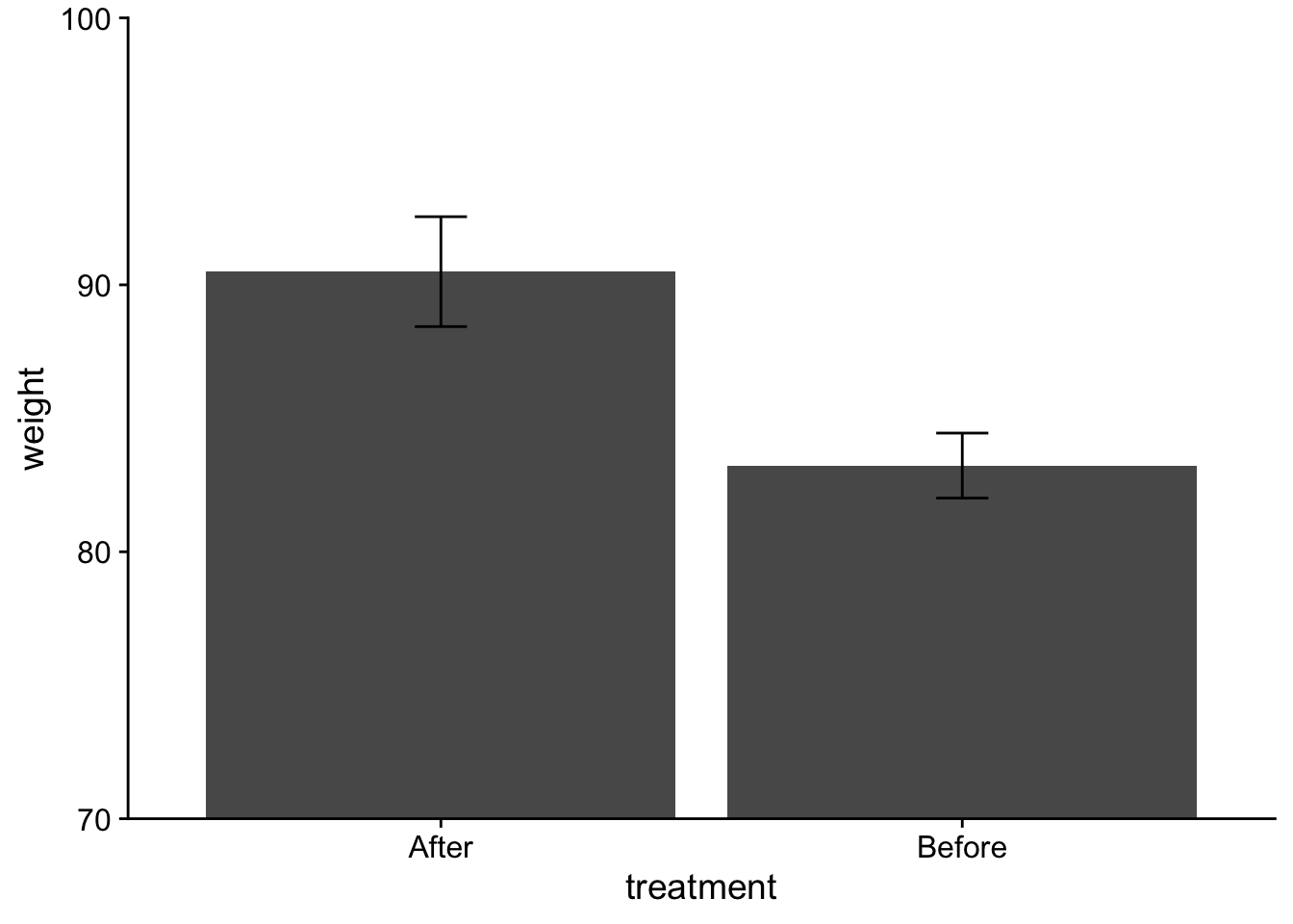
Additionally, to get this into true APA format I would need to adjust my axis labels. Here capitalization is needed. Also, because the weight has a unit measure, I need to be specific about that:
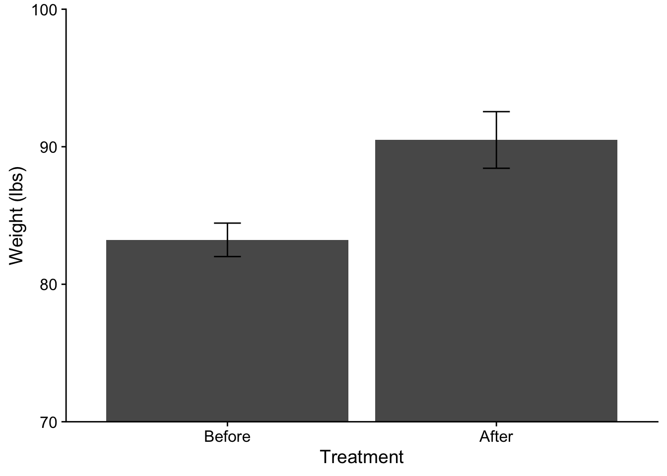
Finally, you may have noticed that the order of Treatment on the plot is opposite of what we might like to logically present. In this case the “After” data comes prior to the “Before” data on the x-axis. This is because R defaults to alphabetical order when loading in data. To correct this I can use scale_x_discrete() and specify the order that I want in limits:
Alternatively I can correct the order of the levels of a factor within the dataframe itself using fct_relevel() (this gets loaded with tidyverse). Note that here I am overwriting the original treatment column. If you do this proceed at your own risk! You could also just mutate a new column if you would rather not overwrite.
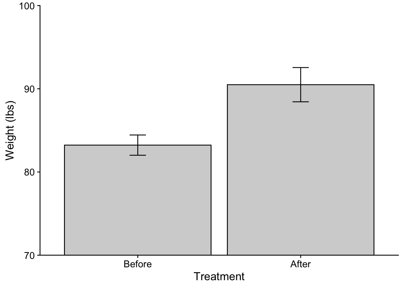
anorexia_data$treatment <-fct_relevel(anorexia_data$treatment, "Before", "After")ggplot(data = anorexia_data, aes(x=treatment, y=weight)) +stat_summary(fun ="mean", geom ="col", fill ="lightgray", color ="black") +# adding some color mods here.stat_summary(fun.data ="mean_se", geom ="errorbar", width = .1) +scale_y_continuous(expand =c(0,0)) +theme_cowplot() +coord_cartesian(ylim =c(70,100)) +xlab("Treatment") +ylab("Weight (lbs)")
# note that I don't have to do the `scale_x_discrete(limits=c("Before","After"))` correction
All good (well maybe check with CJ first)! One other thing to consider (although please do not worry about it here) is the recent argument that when dealing with repeated measures data you need to adjust you error bars. See this pdf by Richard Morey (2005) for more information on this issue. We’ll revisit this issue when running Repeated Measures ANOVA.
27.7 An aside… other types of plots
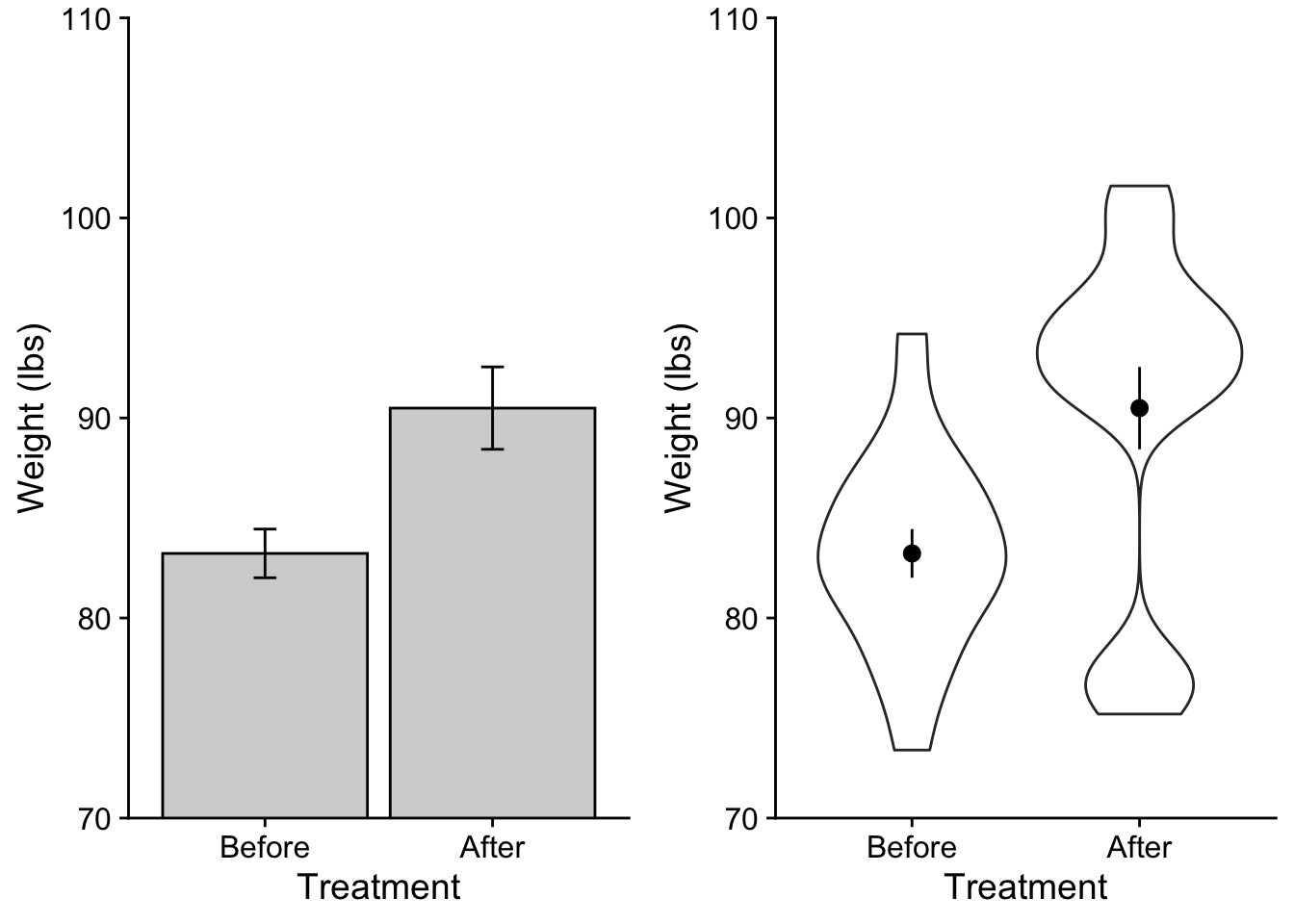
As I mentioned barplots (especially those that use standard error bars) have more recently come under criticism for “hiding” the true name of the data. There is currently a movement to make data more transparent using other kinds of plots that convey more information about your sample. For example let’s contrast out barplot from above with a combination “pointrange” and violin plot. The pointrange simply provides the mean as a point with error bars extending as specified (here I choose standard error). The violin plot is essentially a histogram of the data turned on its side, centered on the mean, and then mirrored… it gives us info about the TRUE distribution of scores.
Let’s take a look side by side
barplot <-ggplot(data = anorexia_data, aes(x=treatment, y=weight)) +stat_summary(fun ="mean", geom ="col", fill ="lightgray", color ="black") +# adding some color mods here.stat_summary(fun.data ="mean_se", geom ="errorbar", width = .1) +scale_y_continuous(expand =c(0,0)) +theme_cowplot() +coord_cartesian(ylim =c(70,110)) +xlab("Treatment") +ylab("Weight (lbs)")# note that order matters. I need to do the violin before the pointrange or else the violin will "paint over" the pointrange.point_violin_plot <-ggplot(data = anorexia_data, aes(x=treatment, y=weight)) +geom_violin() +stat_summary(fun.data ="mean_se", geom ="pointrange", color ="black") +# adding some color mods here.scale_y_continuous(expand =c(0,0)) +theme_cowplot() +coord_cartesian(ylim =c(70,110)) +xlab("Treatment") +ylab("Weight (lbs)")cowplot::plot_grid(barplot, point_violin_plot)
As you can see the second plot gives me more information about what’s truly going on with my data. In this case the After data has an unusual clustering of scores at the lower end of it’s distribution.
27.8 Performing the t-test (Paired sample t-test)
Okay, now that we’ve done all of our preparation, we’re now ready to perform the test. We can do so using the t.test() function. In this case, the experimental question warrants a paired samples t-test.
Since we’ve got long-format data we will use the formula syntax. This reads “predicting changes in weight as a function of treatment.
    Paired t-test

data:  weight by treatment
t = -4.1802, df = 16, p-value = 0.0007072
alternative hypothesis: true mean difference is not equal to 0
95 percent confidence interval:
 -10.948840  -3.580571
sample estimates:
mean difference
      -7.264706
The output provides us with our \(t\) value, the \(df\) and the \(p\) value. It also includes a measure of the 95% CI, and the mean difference. Remember that the null hypothesis is that there is no difference between our two samples. In the case of repeated measures especially, it makes sense to think of this in terms of a difference score of change, where the null is 0. The resulting interpretation is that on average participants’ weight increased 7.26 pounds due to the treatment, with a 95% likelihood that the true mean change is between 3.58 lbs and 10.95 lbs. Important for us is that 0 is not in the 95% CI, reinforcing that there was indeed a non-zero change (rejecting the null).
27.9 One sample \(t\) test:
The data in our example warranted running a paired t-test. However, as noted we can run a t.test() to compare a single sample to a single value. For example it might be reasonable to ask whether or not the 17 adolescent girls that Hand, et al., 1994 treated were different from what would be considered the average weight of a teenaged girl. A quick Google search suggests that the average weight of girls 12-17 in 2002 was 130 lbs. How does this compare to Hand et al.’s participants Before treatment? We can run a one sample t-test to answer this question.
In this case, we don’t need to use the formula convention, we can just use a vector of the data we are interested in and compare it against a population mean mu of 130:
# get the data we wantbeforeTreatment <-filter(anorexia_data,treatment=="Before")# one sample t-testt.test(beforeTreatment$weight, mu =130)
    One Sample t-test

data:  beforeTreatment$weight
t = -38.44, df = 16, p-value < 2.2e-16
alternative hypothesis: true mean is not equal to 130
95 percent confidence interval:
 80.65007 85.80876
sample estimates:
mean of x
 83.22941
Yes, this group of girls was significantly underweight compared to the national average.