pacman::p_load(car,
               cowplot,
               tidyverse,
rstatix)34 The One-way ANOVA
34.1 ANOVAs for comparing means
This week we cover ANOVA. A major emphasis in the material (especially Winter’s optional text) is that ANOVA (much like many of the other tests that we cover in this course) is an extension of the general linear model. In many respects, ANOVA and regression are conceptually identical—whereas in linear regression our predictor variables are typically continuous (or, in some cases ordinal) we usually reserve the term ANOVA for instances when our predictors are discrete or nominal (although it really need not be). This would be the difference say in predicting weight as a function of height (linear regression) in contrast to weight as function of hometown (Dayton, Youngstown, Cleveland, Cincinnati). Given that the assigned readings (and the optional Winter text) do a wonderful job of explaining the underlying principles of ANOVA, I won’t spend too much time here rehashing what is already available there. Both the optional Flora text and the Winter text, especially do an excellent job of demonstrating how even though regression and ANOVA are often treated differently in terms of research focus (e.g., observation v. experimentation) and data focus (correlation/goodness of fit v. comparing means) they are indeed one and the same. Here, my goal is to reinforce this idea using examples in R, as well as providing a practical tutorial that will serve as our entry point into ANOVA.
We typically understand ANOVA as a method for allowing us to compare means from more than two samples. To see how this connects with what we have learned from regression lets use an example dataset. Before proceeding, this walk-through assumes that you have the following packages installed and loaded in R:
34.2 The data
To start, lets download Eysenck’s (1974) study on verbal recall and levels of processing. As described in Howell (2012):
Craik and Lockhart (1972) proposed as a model of memory that the degree to which verbal material is remembered by the subject is a function of the degree to which it was processed when it was initially presented. Thus, for example, if you were trying to memorize a list of words, repeating a word to yourself (a low level of processing) would not lead to as good recall as thinking about the word and trying to form associations between that word and some other word. Eysenck (1974) was interested in testing this model and, more important, in looking to see whether it could help to explain reported differences between young and old subjects in their ability to recall verbal material…
Eysenck randomly assigned 50 subjects between the ages of 55 and 65 years to one of five groups—four incidental-learning groups and one intentional-learning group. (Incidental learning is learning in the absence of the expectation that the material will later need to be recalled.) The Counting group was asked to read through a list of words and simply count the number of letters in each word. This involved the lowest level of processing, because subjects did not need to deal with each word as anything more than a collection of letters. The Rhyming group was asked to read each word and think of a word that rhymed with it. This task involved considering the sound of each word, but not its meaning. The Adjective group had to process the words to the extent of giving an adjective that could reasonably be used to modify each word on the list. The Imagery group was instructed to try to form vivid images of each word. This was assumed to require the deepest level of processing of the four incidental conditions. None of these four groups were told that they would later be asked for recall of the items. Finally, the Intentional group was told to read through the list and to memorize the words for later recall. After subjects had gone through the list of 27 items three times, they were given a sheet of paper and asked to write down all of the words they could remember. If learning involves nothing more than being exposed to the material (the way most of us read a newspaper or, heaven forbid, a class assignment), then the five groups should have shown equal recall—after all, they all saw all of the words. If the level of processing of the material is important, then there should have been noticeable differences among the group means.
We can download this dataset using the following code:
dataset <- read_delim("https://www.uvm.edu/~statdhtx/methods8/DataFiles/Ex11-1.dat",
                      delim = "\t")
Rows: 50 Columns: 2
── Column specification ────────────────────────────────────────────────────────
Delimiter: "\t"
dbl (2): GROUP, RECALL
ℹ Use `spec()` to retrieve the full column specification for this data.
ℹ Specify the column types or set `show_col_types = FALSE` to quiet this message.dataset# A tibble: 50 × 2
GROUP RECALL
<dbl> <dbl>
1 1 9
2 1 8
3 1 6
4 1 8
5 1 10
6 1 4
7 1 6
8 1 5
9 1 7
10 1 7
# ℹ 40 more rows34.3 Getting the data in order
Although the focus for this course is conceptual and applied knowledge of statistics, I again want to be mindful of the practice of data analysis. That is, in the real world, you’ll be asked to do some data wrangling, or getting your data in the right format and containing the right information to properly proceed with analysis. When looking at this data, two important things jump out that we might want to address: (1) there is no column indicating participant ID. and (2) the data is numerically coded. A little bit about each of these points.
34.3.1 The importance of a participant ID column
Depending on what statistical software you use, including a Participant ID column varies in its importance. For building statistical models in R that involve categorical data, including designs that that test within and across subjects making sure that you have Participant IDs coded is vitally important. Ideally this will already be done before you import your data, but on the case that it’s not you need to add a column specifying participant ID. How you do this will depend on what format your data is in (Wide v. Long) and whether you have a repeated-measures design (multiple measures from each participant).
** I grant that it might be useful to use you Excel ninja skills here and get everything in its right place before importing, but will assume that you want to stay in an R environment.
In this case, our data is in long format and we have a between subjects design. That is every line represents a single measure of a participant and every participant is represented only once. In this case we can just assign a unique number to each participant / row. In most cases this is a simple as assigning participant numbers {1,2,3…n}. An easy way to do this is to use the row_number() function. The row_number() function simply says to create numbers in sequence corresponding to the rows in your table.
dataset <- dataset %>% mutate(PartID = row_number())
dataset
# A tibble: 50 × 3
GROUP RECALL PartID
<dbl> <dbl> <int>
1 1 9 1
2 1 8 2
3 1 6 3
4 1 8 4
5 1 10 5
6 1 4 6
7 1 6 7
8 1 5 8
9 1 7 9
10 1 7 10
# ℹ 40 more rowsFWIW, if you have the same compulsion that I do and insist that your PartID column is first in your dataset this can be solved using select. Here, I’m saying put PartID first and then follow it with everything() else.
dataset <- dataset %>% select(PartID, everything())
dataset %>% head()
# A tibble: 6 × 3
PartID GROUP RECALL
<int> <dbl> <dbl>
1 1 1 9
2 2 1 8
3 3 1 6
4 4 1 8
5 5 1 10
6 6 1 4OK. That’s addressed. Now onto issue #2.
34.3.2 Recoding the factors (if number coded)
As we can see the data is number coded. In this case,
1 = ‘Counting’,
2 = ‘Rhyming’,
3 = ‘Adjective’,
4 = ‘Imagery’ and
5 = ‘Intentional’
My advice for what to do if you get dummy coded data is to create a corresponding column in your data set that contains the factors in nominal (name) format.
We can use the fct_recode() function to reassign the number variables into categorical names. Importantly, if your data is numerically coded you would need to convert it into a factor before applying the function. Notice in the code below I am applying the as.factor() function to GROUP within the fct_recode call:
# assigning the appropriate names for the dummy codes
dataset <-
  dataset %>%
  mutate(GROUP_FACTOR = fct_recode(factor(GROUP),
                                 Counting = "1",
                                 Rhyming = "2",
                                 Adjective = "3",
                                 Imagery = "4",
                                 Intentional = "5"
                                 )
  )

head(dataset)
# A tibble: 6 × 4
PartID GROUP RECALL GROUP_FACTOR
<int> <dbl> <dbl> <fct>
1 1 1 9 Counting
2 2 1 8 Counting
3 3 1 6 Counting
4 4 1 8 Counting
5 5 1 10 Counting
6 6 1 4 Counting I now have a column of data that treats my originally numerically coded IVs as factors. This is important as it will allow me to use the GROUP_FACTOR column as a predictor in my model.
34.3.3 Renaming column headers (optional)
And now, just to be clear, let’s rename the original GROUP to GROUP_NUM. This can be accomplished by using the dplyr::rename() function.
# The template is rename(NEW_NAME = OLD_NAME)
dataset <- dataset %>% rename(GROUP_NUM = GROUP)
dataset
# A tibble: 50 × 4
PartID GROUP_NUM RECALL GROUP_FACTOR
<int> <dbl> <dbl> <fct>
1 1 1 9 Counting
2 2 1 8 Counting
3 3 1 6 Counting
4 4 1 8 Counting
5 5 1 10 Counting
6 6 1 4 Counting
7 7 1 6 Counting
8 8 1 5 Counting
9 9 1 7 Counting
10 10 1 7 Counting
# ℹ 40 more rowsCheck out this link for info on how to rename multiple columns at once using names() or dplyr::rename() from the tidyverse.
34.3.4 Reordering your levels
One important question you should ask before you look at your data is “what is your control (group, condition)”. Proper experimentation requires a proper control in order to properly isolate the influence of the manipulation (that’s a lot of “proper”s). Here, the best candidates for our control group might either be “Counting” or “Intentional”, depending on how the original problem was approached. If the larger comparison involved “Intentional v. incidental” learning for recall, then the “Intentional” group serves best as your control. If the original question involved levels of processing, then “Counting”” (theoretically the lowest level of incidental processing) is best. Here I am assuming the latter (although I believe theoretically Eysenck originally was interested in the former).
I bring this up, as its typically best to ensure that your control is entered first into the ANOVA model. To check the order of your levels, you may simply:
levels(dataset$GROUP_FACTOR)[1] "Counting" "Rhyming" "Adjective" "Imagery" "Intentional"Here we see that “Counting” is first and will therefore be entered first into the model.
Assuming that we wanted to reorder the sequence, say to have Intentional as the control, then we might simply use fct_relevel():
dataset <- dataset %>%
  mutate(GROUP_FACTOR = fct_relevel(GROUP_FACTOR, "Intentional"))

# rechecking the order of the levels
levels(dataset$GROUP_FACTOR)
[1] "Intentional" "Counting" "Rhyming" "Adjective" "Imagery" Note that with fct_relevel() whatever level(s) I list get moved to the front of the line. In this case I just bumped Intentional up while keeping the remaining levels ordered the same.
However, I liked the original order, so let’s change it back:
dataset <- dataset %>%
  mutate(GROUP_FACTOR = fct_relevel(GROUP_FACTOR,
                                    "Counting",
                                    "Rhyming",
                                    "Adjective",
                                    "Imagery",
                                    "Intentional"))

levels(dataset$GROUP_FACTOR)
[1] "Counting" "Rhyming" "Adjective" "Imagery" "Intentional"That’s better. Why the order is important will be made clear later in this write up. For now, think back to our example in class of running a t-test using lm(). You may recall that the group level that was first entered into the model served as the model intercept where the second group level was expressed in terms of the slope of the line (beta). A similar output will be happening here.
So the data structure looks good.
One last little bit of ninja-ing. If you wanted to save a particular R object to be used later on you can use the write_rds() function (from tidyverse). I’m going to save dataset as I’ve cleaned it up so that I can use it in the next walkthrough.
write_rds(dataset,'clean_dataset.rds')Alternatively, if I wan’t to save it as something I can look at outside of R I can use write.csv():
write.csv(dataset,'clean_dataset.csv')Onward to the analysis!!!!
34.4 Assumptions for ANOVA
34.4.1 Checking the normality assumption, OPTION 1 raw data by group
To check the distribution of outcomes in ANOVA, you have two options. The first would be to check the distribution of outcomes for EACH group/condition independently. In the case of the example dataset we could get info related to the skew and kurtosis of RECALL for each GROUP_FACTOR using some of the dplyr functions you learned in DataCamp:
dataset %>%
  group_by(GROUP_FACTOR) %>%
  summarise(
    skew = psych::skew(RECALL),
    kurt = psych::kurtosi(RECALL)
  )
# A tibble: 5 × 3
GROUP_FACTOR skew kurt
<fct> <dbl> <dbl>
1 Counting 0 -1.22
2 Rhyming 0.178 -0.398
3 Adjective -0.657 -0.841
4 Imagery 0.994 -0.532
5 Intentional 0.0458 -0.474If we wanted to perform more extensive methods like the shapiro test, we could also use this method:
dataset %>%
  group_by(GROUP_FACTOR) %>%
  rstatix::shapiro_test(RECALL)
# A tibble: 5 × 4
GROUP_FACTOR variable statistic p
<fct> <chr> <dbl> <dbl>
1 Counting RECALL 0.984 0.982
2 Rhyming RECALL 0.930 0.450
3 Adjective RECALL 0.906 0.255
4 Imagery RECALL 0.820 0.0251
5 Intentional RECALL 0.943 0.591 BUT, this is a lot of work. And it’s not very efficient. So let’s look at the second option.
34.4.2 Checking the normality assumption, OPTION 2, the better way: Look at the residuals.
Although group_by() may or may not make life easier for you in this test case, things rapidly become more complicated when attempting to check normality by condition. For example if you’re running a 2×3×3 mixed effect ANOVA, you would need to run through 18 conditions!!! So what to do?!?!?!
A simpler alternative is to run you model and analyze your residuals. This web link does a nice and quick job of explaining the logic.
In this case we would run our ANOVA model using lm (see told you its all the same)
dataset_aov <- lm(RECALL~GROUP_FACTOR, data=dataset)Congrats, you’ve just run an ANOVA, but for now we aren’t interested in the results from the model. Remember from a few weeks back we noted that we can use the performance package to check the overall model assumptions (including normality)
pacman::p_load(performance)
performance::check_model(dataset_aov)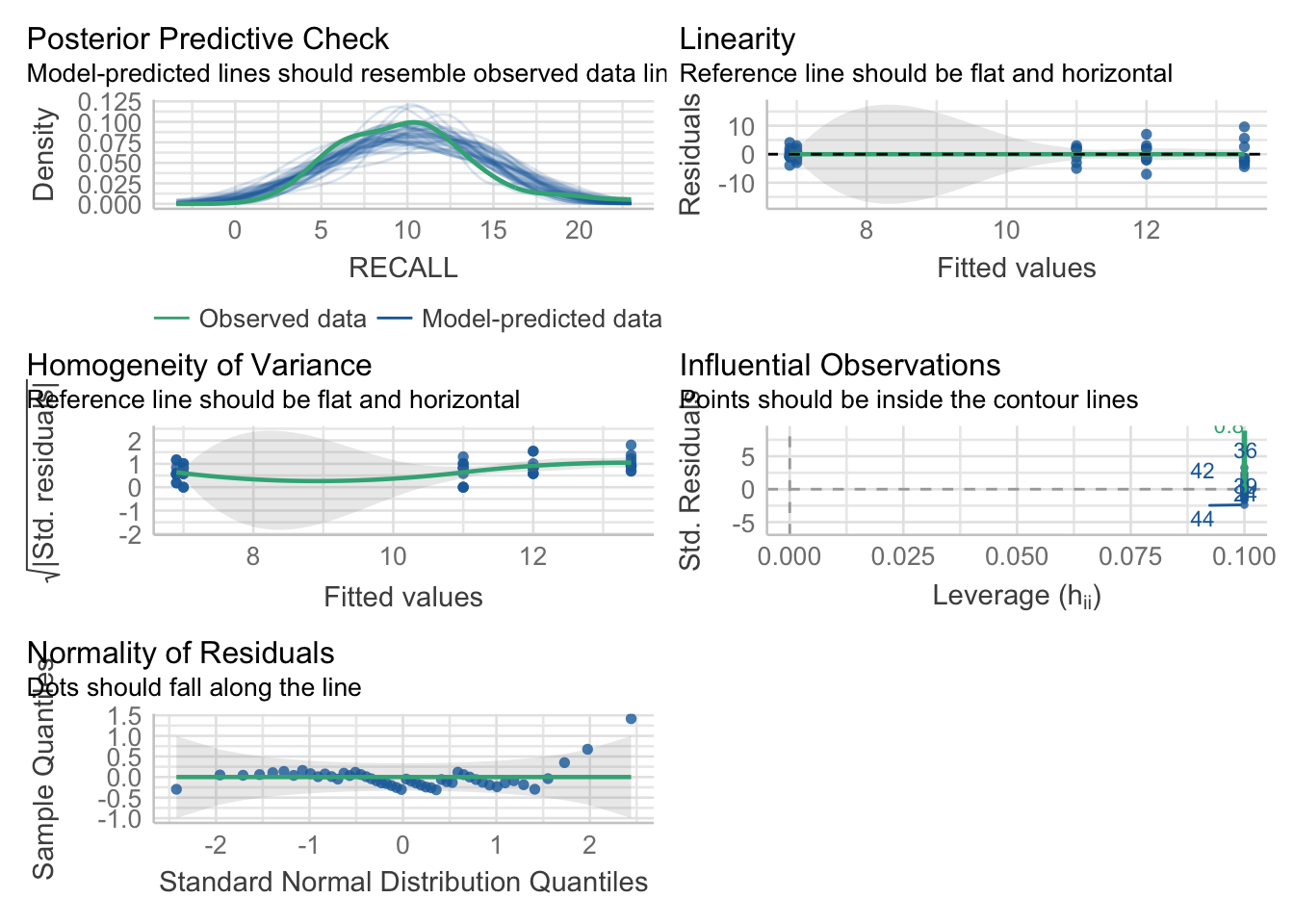
And for the more explicit normality tests:
performance::check_normality(dataset_aov)OK: residuals appear as normally distributed (p = 0.086).# if we wanted to focus on the qqplot:
performance::check_normality(dataset_aov) %>% plot("qq")
So, between OPTION 1 and OPTION 2, I’d recommend typically going with OPTION 2. Especially as your ANOVA designs become more complex. `
34.4.3 Homogeneity of Variance
Another assumption of ANOVA is the homogeneity of variance between groups. An easy-way to get an eyeball test of this assumption is two perform a box plot of the data. Here I am performing this plot using ggplot2:
ggplot(data =dataset, aes(x=GROUP_FACTOR,y=RECALL)) +
  geom_boxplot()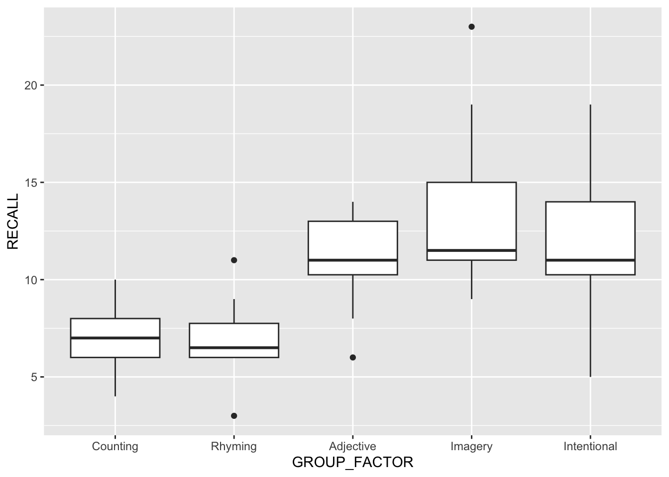
Huge differences in the IQR regions may be a clue that the homogeneity assumption is violated. We can run more specific tests in R including the Levene Test and Fligner-Killeen Test of Homogeneity of Variances. You are familiar with the Levene Test from a few weeks ago. The Figner-Killeen Test is offered as an alternative if you are concerned with violations of the normality assumption.
As is typically the case \(p<.05\) indicates a violation of this assumption:
# Bartlet Test of Homogeneity of Variances
performance::check_homogeneity(dataset_aov)
Warning: Variances differ between groups (Bartlett Test, p = 0.042).# Fligner-Killeen Test of Homogeneity of Variances
performance::check_homogeneity(dataset_aov, method = "fligner")OK: There is not clear evidence for different variances across groups (Fligner-Killeen Test, p = 0.741).34.4.4 What to do if the assumptions are violated?
If either assumption is violated, one option that you have is to transform you data. We’ve talked several times in class about the pros and cons of doing this, and there are several resources that provide examples of how this is done. Another option is to use a non-parametric test such as the Kruskal-Wallis Test if the data is not normal, or Welch’s ANOVA is the variances are not homogeneous. That said, one of reasons that ANOVA is so popular is that it has been demonstrated to be robust in the face of violated assumptions (as long as the sample sizes are equal). For example, in Design and Analysis of Experiments (1999, p. 112) Dean & Voss argue that the maximum group variance may be as high as 3× the minimum group variance without any issue. With this in mind, a question (gray area) before us is how much of a violation is there in the data? And if not so much, you may be fine just running an ANOVA regardless. Let’s check the variance of the groups in our example:
dataset %>%
  group_by(GROUP_FACTOR) %>%
  summarise(
    var = var(RECALL)
  )
# A tibble: 5 × 2
GROUP_FACTOR var
<fct> <dbl>
1 Counting 3.33
2 Rhyming 4.54
3 Adjective 6.22
4 Imagery 20.3
5 Intentional 14 Looks like in this example, we may still have an issue. For now I’m going to ignore it, but you should be aware that this is a potential issue.
34.5 Running the ANOVA in R using aov() or lm()
There are many, many ways to build an ANOVA model in R. This week we will concentrate on aov() which is the standard method, as well as the lm() method that you have used before, just to reinforce that ANOVA and regression are one in the same. In fact, SPOILER ALERT, aov() is just a fancy wrapper for lm().
Like lm() from weeks past, aov() asks us to enter our dependent and independent variables into the model in the formula format DV ~ IVs. In this case, we only have a single IV, GROUP_FACTOR. Thus our model is:
aov_model <- aov(RECALL~GROUP_FACTOR,data = dataset)From here, we can use the anova() function to give us our ANOVA table.
anova(aov_model)Analysis of Variance Table
Response: RECALL
Df Sum Sq Mean Sq F value Pr(>F)
GROUP_FACTOR 4 351.52 87.880 9.0848 1.815e-05 ***
Residuals 45 435.30 9.673
---
Signif. codes: 0 '***' 0.001 '**' 0.01 '*' 0.05 '.' 0.1 ' ' 1Note however that this output is fairly limited. Yes, it give us our \(F\) value and many of the crucial relevant statistics, but notably it does not provide us with our effect size. Instead, we can use a function from the rstatix package. This has two added benefits:
- it gives us an effect size measure and
- it also allows us to adjust how our Sums of Squares are calculated. This isn’t important for simple One-way ANOVA, but see the Field text, Jane Superbrain 11.1 for an explanation.
Here is an example. Note that we are using the type = 3 argument to specify the type of SS calculation we want. This is the default for rstatix::anova_test(). I’m also specifying that I want general eta squared \(\eta^2\) as my effect size measure.
rstatix::anova_test(aov_model, type = 3, effect.size = "ges")ANOVA Table (type III tests)
Effect DFn DFd F p p<.05 ges
1 GROUP_FACTOR 4 45 9.085 1.82e-05 * 0.447FWIW… a super-duper comprehensive anova table can be obtained by submitting our aov_model to sjstats::anova_stats(), which gives us our effect sizes as well! This function calculates eta-squared (\(\eta^2\)), partial-eta-squared (\(\eta_p^2\)), omega squared (\(\omega^2\)) and partial omega-squared (\(\omega_p^2\)) as well as Cohen’s f. Typically for One-Way ANOVA psychologists report eta-squared (\(\eta^2\)), though there are arguments that omega squared (\(\omega^2\)) may be the more preferred measure.
pacman::p_load(kableExtra)
pacman::p_load(sjstats)
sjstats::anova_stats(aov_model) %>%
  kbl(caption = "Super ANOVA table") %>%
kable_classic(full_width = F, html_font = "Cambria")| term | df | sumsq | meansq | statistic | p.value | etasq | partial.etasq | omegasq | partial.omegasq | epsilonsq | cohens.f | power | |
|---|---|---|---|---|---|---|---|---|---|---|---|---|---|
| GROUP_FACTOR | GROUP_FACTOR | 4 | 351.52 | 87.880 | 9.085 | 0 | 0.447 | 0.447 | 0.393 | 0.393 | 0.398 | 0.899 | 0.999 |
| ...2 | Residuals | 45 | 435.30 | 9.673 | NA | NA | NA | NA | NA | NA | NA | NA | NA |
I typically don’t recommend using sjstats::anova_stats() unless you are looking for these more exotic effect sizes.
34.6 Plotting your data
For publication quality ANOVA plots, there are typically three acceptable plots used to convey your results, box plots, bar plots, and line plots. As the ANOVA become more complex, we tend towards using line plots (box plots and bar plots may become very busy in complex designs). Unless there are other compelling reasons we tend to plot the means (although note that box plots usually give you medians). Since you have already produced box plots and barplots, I’ll show examples of how to do a line plot.
To create a line plot with points at the means and error lines representing the 95% CI (known as a point range), we can use call that you are familiar with and a new geom pointrange. Whats nice about point range is that it allows you to create your points and the error bars all in a single line.
ggplot2::ggplot(data =dataset,mapping = aes(x = GROUP_FACTOR, y = RECALL)) +
  stat_summary(fun.data = mean_cl_normal,
               size=1,
               color="black",
               geom="pointrange")
Now to add the lines to this plot. For this you will need another stat_summary() line specifying that the vertices of the lines should be the means, fun = mean and a parameter that specifies how the lines should be grouped. Since we have a One-way ANOVA, group=1. When we built to more complex designs you may elect to group=FACTOR_NAME. Something like this is useful to say make some lines dashed and some lines solid according to levels on a factor. More on this in two weeks when we get to factorial ANOVA.
While we’re at it let’s fix those axes titles. We can use the functions xlab() and ylab() to do so.
# this is from before, saving as object "p"
p <- ggplot2::ggplot(data =dataset,mapping = aes(x = GROUP_FACTOR, y = RECALL)) +
  stat_summary(fun.data = mean_cl_normal,
               size=1,
               color="black",
               geom="pointrange") +
  # adding lines
  stat_summary(fun = mean,
               size = 1,
               color = "black",
               mapping=aes(group=1),
               geom="line") +
  # and fixing the axis titles:
  xlab("Group")+ylab("Words recalled")
Warning: Using `size` aesthetic for lines was deprecated in ggplot2 3.4.0.
ℹ Please use `linewidth` instead.show(p)
Finally, for aesthetic reasons you may elect to expand the y-axis. For example to make the range of y-axis values (0,20) and use cowplot::theme_cowplot() to make the plot look a little more APA friendly.
pacman::p_load(cowplot)
p + expand_limits(y=c(0,20)) + theme_cowplot()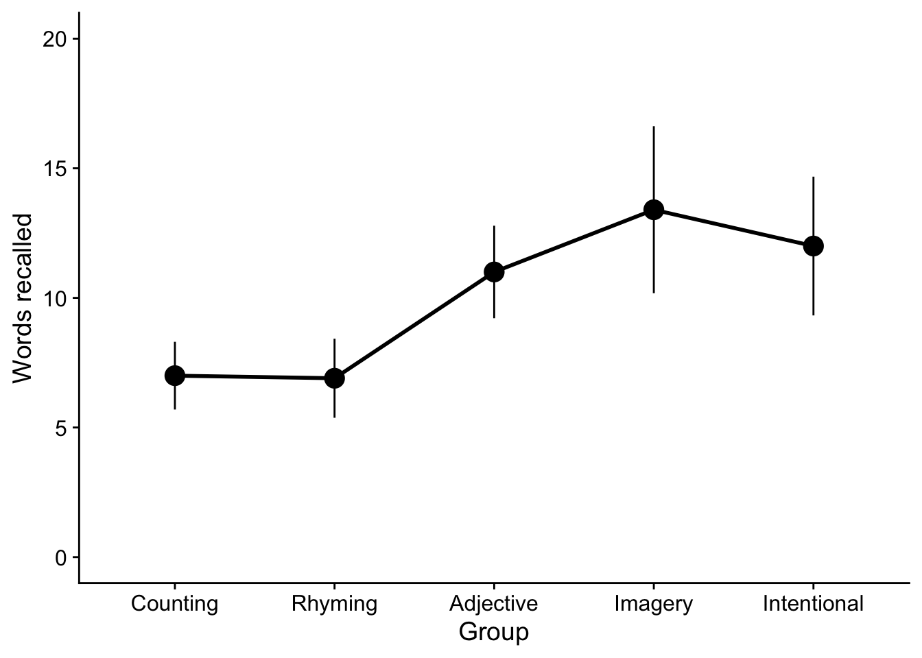
That being said, this data probably lends itself to a bar plot. This is similar to how you built your bar plots from as when doing a t-test. As a matter of fact, as practice why don’t you give that a shot right now. I’ll wait.
34.7 Reporting your data / the write up
There are two components to reporting your one-way ANOVA. First, You need to report your output as related to the test:
- the F value,
- the degrees of freedom (between and within),
- the p-value
- effect size: typically with between-effects ANOVA we report eta squared.
Second, as we typically focus on means with ANOVA, it is typically a good idea to report means and some report of of the distribution of each group (typically either standard deviation or standard error; although 95% CI may be useful in certain scenarios).
So for example reporting the Rhyming group:
- M ± SD: 6.90 ± 2.13
- M ± SE: 6.90 ± 0.67
34.8 What the one-way ANOVA tells you
While it may be useful to report the means, you need to be mindful of what the omnibus ANOVA tells you. Remember, that the the null hypothesis of the omnibus ANOVA is that “there are no differences between observed means”. Our significant result tells us that there are differences between our means, but does not tell us what those specific differences are. So while it may be useful to report general relationships, e.g., “Recall for people in the Intentional group tended to be greater than for the Counting group” you cannot say definitively “Recall was significantly greater for the Intentional Group”. Typically when you only have tested the omnibus ANOVA, you only speak in generalities (e.g., “Recall tended to increase with level of processing.”)
Always be mindful that you don’t over interpret your data.
34.9 Running an ANOVA using lm() (it’s a regression afterall)
Now that we’ve got practical matters out of the way, I want to take some time to dig a little deeper into the connections between ANOVA this week and our work on correlations and regressions in the past.
As we’ve already mentioned (and spent time discussing in class) ANOVA is just an extension of the simple linear model that we covered last week, where ANOVA is used when our predictors are discrete. In fact aov() is simply a wrapper for the lm() function that we used last week. For example, let’s run our model using lm() and then pipe it into rstatix::anova_test().
lm_model <- lm(RECALL~GROUP_FACTOR, data=dataset)
rstatix::anova_test(lm_model)
ANOVA Table (type II tests)
Effect DFn DFd F p p<.05 ges
1 GROUP_FACTOR 4 45 9.085 1.82e-05 * 0.447All aov() does is take an lm object and produce an ANOVA table from the results. If we were simply to look at the lm() model we see that it gives us the info in our ANOVA table at the end of the summary, including the F-statistic (9.085), the degrees of freedom (4 and 45) and the p-value (1.815e-05):
lm(RECALL~GROUP_FACTOR, data=dataset) %>% summary()
Call:
lm(formula = RECALL ~ GROUP_FACTOR, data = dataset)

Residuals:
   Min     1Q Median     3Q    Max
 -7.00  -1.85  -0.45   2.00   9.60

Coefficients:
                        Estimate Std. Error t value Pr(>|t|)
(Intercept)               7.0000     0.9835   7.117 6.83e-09 ***
GROUP_FACTORRhyming      -0.1000     1.3909  -0.072 0.943004
GROUP_FACTORAdjective     4.0000     1.3909   2.876 0.006138 **
GROUP_FACTORImagery       6.4000     1.3909   4.601 3.43e-05 ***
GROUP_FACTORIntentional   5.0000     1.3909   3.595 0.000802 ***
---
Signif. codes:  0 '***' 0.001 '**' 0.01 '*' 0.05 '.' 0.1 ' ' 1

Residual standard error: 3.11 on 45 degrees of freedom
Multiple R-squared:  0.4468,    Adjusted R-squared:  0.3976
F-statistic: 9.085 on 4 and 45 DF,  p-value: 1.815e-05
Taking a look at this output, we see that the lm() model also gives us a lot of other additional useful info. For example the \(R^2\) of the model may be understood as the effect size of the ANOVA. However, when we report it for One-Way ANOVA we express it as… dun, dun, dunnnn… eta-squared!!, or \(\eta^2\).
One more time with feeling, for simple oneway ANOVA, \(R^2\) and \(\eta^2\) are the same damn thing!!
Zooming in on the coefficients:
                        Estimate Std. Error     t value     Pr(>|t|)
(Intercept)                  7.0  0.9835311  7.11721300 6.830993e-09
GROUP_FACTORRhyming         -0.1  1.3909230 -0.07189471 9.430043e-01
GROUP_FACTORAdjective        4.0  1.3909230  2.87578833 6.137702e-03
GROUP_FACTORImagery          6.4  1.3909230  4.60126133 3.425167e-05
GROUP_FACTORIntentional      5.0  1.3909230  3.59473541 8.019114e-04
We see information about the means of each group relative to the (Intercept). This is why I stressed earlier that it may be useful to rearrange the order of your levels such that R enters your control group into the model first. In this case, the first predictor entered is assigned to the (Intercept). The remaining predictors in the model are then presented relative to the first. Since we entered “Counting” first, the estimate of the (Intercept) represents its mean. The means for each remaining group are the sum of its estimate coefficient and the (Intercept). So for example the mean of the Rhyming group is \((-0.1)+(7.0)=6.9\).
The coefficients section also gives us one other useful bit of information, the \(t\)-values of the estimate. As we learned a few weeks ago, for a simple regression the beta coefficient gives us information about the slope of the regression line and the corresponding \(t\)-value is a test of the null \(beta=0\). So for a simple regression this tells us if our slope is significantly different from 0.
A similar logic applies to the ANOVA model. As I mentioned above, deriving the means of each level of our IV is a matter of summing the (Intercept) and the beta estimate for that level. It should be apparent, then, that the beta estimates here represent the slope of a line that between the intercept and the mean of the level (where the distance between the predictor and coefficient is treated as a unit 1). Therefore, a significant \(t\)-value for beta tells us that the slope between the two means is significant, or that those two means are significantly different from one another.
Keep in mind the only comparisons that are being made here are between the individual levels of our IV and the control (Intercept). So while this output allows us to make a claim about the difference between the means of the Counting (Intercept) group compared to each of the other groups, it does not allow us to make a claim about differences between our other levels. For example no information about a statistical test of differences between the Rhyming and Imagery groups is conveyed here. However, assuming you are interested in deviations from your control, you can get info here quickly. There is a caveat here, in that our alpha criterion will need to be adjusted to be more conservative than .05. More on this next week.
34.10 Reporting your results.
34.10.1 Reporting just the ANOVA
For this week’s assignment, you are going to be asked to simply report the ANOVA. In future weeks you will see that simply reporting the ANOVA is not the end of your analysis, but only the beginning of additional, necessary follow-ups. But that is for next week, for now let’s take a look at what one might expect to be reported in an ANOVA write-up.
Given our example:
- words RECALL is our dependent measure
- GROUP_FACTOR is our independent variable, with five levels (or groups).
rstatix::anova_test(aov_model, effect.size = "ges")ANOVA Table (type II tests)
Effect DFn DFd F p p<.05 ges
1 GROUP_FACTOR 4 45 9.085 1.82e-05 * 0.447From this table, we need our:
- df: 4 and 45
- F-statistic: 9.085
- p.value: <.001
- ges: .45
Taking all of this info, and plugging into a write-up template (inserted points in bold):
“We hypothesized that different types of memorization strategies would result in different levels of memorization between our five groups, as measured by the number of words recalled. To test this hypothesis we conducted a One-way Analysis of Variance. Our analysis revealed a significant effect for Groups, F(4, 45) = 9.08, p < .001, \(\eta^2\) = .45; see Figure 1.”
For now, this is all you can say with only running a One-way ANOVA using this method, and that’s all I would want for the homework for this week.
34.10.2 Reporting the ANOVA, lm() output
Let’s revisit the lm() output. Recall that the lm() method gives us the added benefit of comparing each level of the GROUP_FACTOR to the control level. This is what’s known as treatment contrasts (see Winter, Chapter 7). In this case, our control level is Counting and every other level (group) is compared against Counting and captured in the resulting beta coefficients:
aov_model_lm <- lm(RECALL~GROUP_FACTOR, data = dataset)
summary(aov_model_lm)
Call:
lm(formula = RECALL ~ GROUP_FACTOR, data = dataset)

Residuals:
   Min     1Q Median     3Q    Max
 -7.00  -1.85  -0.45   2.00   9.60

Coefficients:
                        Estimate Std. Error t value Pr(>|t|)
(Intercept)               7.0000     0.9835   7.117 6.83e-09 ***
GROUP_FACTORRhyming      -0.1000     1.3909  -0.072 0.943004
GROUP_FACTORAdjective     4.0000     1.3909   2.876 0.006138 **
GROUP_FACTORImagery       6.4000     1.3909   4.601 3.43e-05 ***
GROUP_FACTORIntentional   5.0000     1.3909   3.595 0.000802 ***
---
Signif. codes:  0 '***' 0.001 '**' 0.01 '*' 0.05 '.' 0.1 ' ' 1

Residual standard error: 3.11 on 45 degrees of freedom
Multiple R-squared:  0.4468,    Adjusted R-squared:  0.3976
F-statistic: 9.085 on 4 and 45 DF,  p-value: 1.815e-05
From this summary output we would not only extract our F-statistic, df, p-value and R-squared (remember that \(R^2\) is \(\eta^2\)) as we do for the previous write-up, but now we can talk about differences between the other levels and Counting as expressed as a t value (we are running t-tests).
In some cases you may want to also report the means of each of Groups. We then combine this info with info related to the means and standard errors:
dataset %>%
  group_by(GROUP_FACTOR) %>%
  rstatix::get_summary_stats(RECALL, type = "mean_se")
# A tibble: 5 × 5
GROUP_FACTOR variable n mean se
<fct> <fct> <dbl> <dbl> <dbl>
1 Counting RECALL 10 7 0.577
2 Rhyming RECALL 10 6.9 0.674
3 Adjective RECALL 10 11 0.789
4 Imagery RECALL 10 13.4 1.42
5 Intentional RECALL 10 12 1.18 Putting all of this info together, we might say:
“We hypothesized that different types of memorization strategies would result in different levels of memorization between our five groups, as measured by the number of words recalled. To test this hypothesis we conducted a One-way Analysis of Variance. Our analysis revealed a significant effect for Groups, F(4, 45) = 9.08, p < .001, \(\eta^2\) = .45. As can be seen in Figure 1, we found that the average number of words recalled for the Adjective (\(M\) = 11.0, SE = 0.79; \(t\)(45) = 2.88), Imagery (\(M\) = 13.4, SE = 1.42; \(t\)(45) = 4.60), and Intentional (\(M\) = 12.0, SE = 1.18; \(t\)(45) = 3.60) memorization groups were all greater than the Counting group (\(M\) = 7.0, SE = 0.58); ps < .01”.
- note that I find it acceptable to lump the p-values together in this manner when doing multiple comparisons, as we are doing here.
In both cases BE SURE TO PRODUCE A CAMERA READY FIGURE and REFER TO IT IN THE TEXT!!!