pacman::p_load(tidyverse)16 Building intuitions about standardization & probability
16.1 A few words on where we are at so far…
In the previous walkthrough, we discussed the normal distribution. We also noted that standardization was an important concept and method that was based upon the normal distribution. Standardization is the process of transforming scores in a distribution so that they share a common scale. This in turn allows us to compare scores from different scales to one another (for example IQ to GRE to SAT). Rather than raw scores, these measures can be expressed and compared using starndard score. This is often done by converting scores into z-scores, and is especially important when using scales that have different ranges as predictors in the same model (more on that when we get to correlation and regression).
For now, we can note that the standard normal distribution, often represented as \(N(0,1)\), is a special case of the normal distribution with a mean (\(\mu\)) of 0 and a standard deviation (\(\sigma\)) of 1. Assuming that you have a set of scores \({X_1, X_2, \ldots, X_N}\), to convert these scores into a standard normal distribution, you would calculate the z-scores for each data point using the formula:
\[ z = \frac{X - \mu}{\sigma} \]
Where \(X\) is the individual data point, \(\mu\) is the mean of the dataset, and \(\sigma\) is the standard deviation. By converting each data point into its corresponding z-score, you create a new distribution of scores that is centered around zero and has a standard deviation of 1. This process, called standardization, allows for easier comparison between different distributions and facilitates statistical analysis. Once the data is standardized, it becomes possible to understand and interpret individual scores relative to the entire dataset. Moreover, with the data in this form, you can use tables or software that are calibrated for the standard normal distribution to find probabilities, critical values, or to conduct hypothesis tests.
You may notice that the concept of the z-score is closely related to probability distributions. Recalling the Empirical Rule, we have already loosely talked about our distribution of scores (in that case raw scores) as a distance from the mean with respect to standard deviations. That is, we talked in terms of about 68% of scores falling within 1 standard deviation of the mean, 95% within 2 standard deviations, etc.
\(Z\)-scores are expressing this idea with finer precision. Specifically, the area under the curve of the standard normal distribution gives probabilities associated with \(z\)-scores, where 68% fall within one standard deviation (\(z = \pm 1\)), 95% fall within 1.96 standard deviations (\(z = \pm 1.96\)), etc.
We can do wonderful things the standard distribution, including assessing the probability of an obtained value within that distribution. For example, we know that a z-score greater than 1.96 has a p-value of less than .05. Given what you know about tests for significance, you can bet your bottom dollar that this is crucial for us!!
Before jumping to that, however, lets build some intuitions about probability. There are several tools at our disposal for simulating and understanding probability as it relates to the normal and standard distributions in R. First we need to load in our packages:
16.2 Simulating distributions
For example, we can generate a random, normal distribution, we’ll name it normDist using the rnorm() function:
# setting the seed so our "random" numbers are the same
set.seed(20)
# make 200 observations with mean = 100 & sd = 15
normDist <- rnorm(n = 200, mean = 100, sd = 15)
# make a quick histogram
hist(normDist) 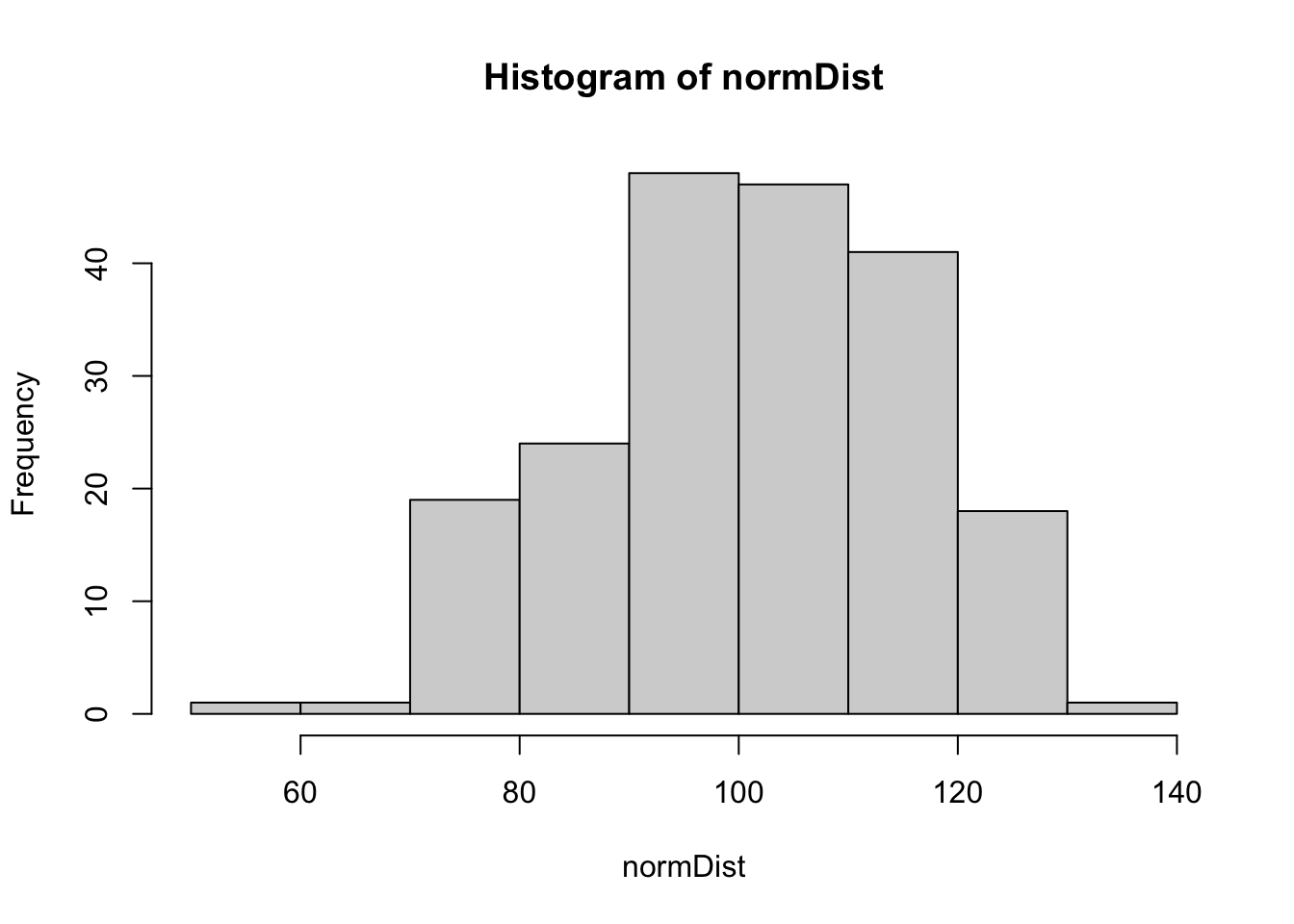
and we can convert these normDist scores to a standard distribution by submitting them to scale():
standardDist <- scale(normDist) # transform to z-scores
hist(standardDist) # make a quick histogram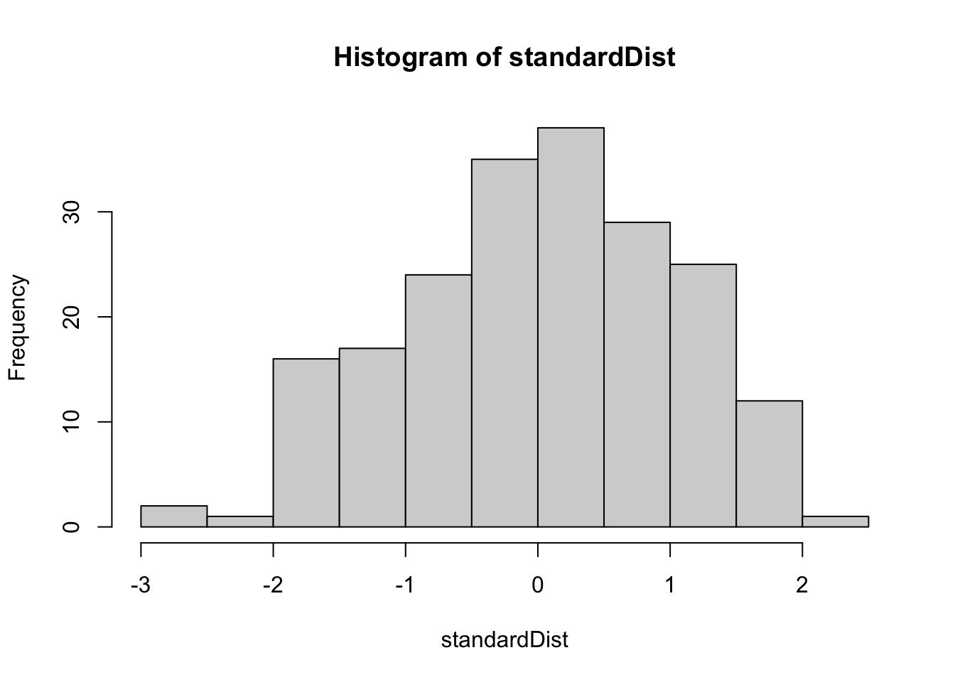
We can use pnorm() to assess the cumulative probability of a given score. In other words what is the likelihood of getting that score or lower in our distribution. The pnorm() function defaults to the standard distribution, that is it assumes that you have a mean=0 and sd=1. Taking a look at its input parameters:
pnorm(q, mean, sd, lower.tail) where q is the value in question; mean and sd relate known values of the distribution, and lower.tail is a logical telling you whether you are looking at the cumulative probability (TRUE) or looking at the upper tail (FALSE). For example, run each line separately and see the output.
# 1. prob of z score of 1.96 or less
pnorm(q = 1.96)
[1] 0.9750021# 2. prob of z score of 1.96 or greater
pnorm(q = 1.96, lower.tail = FALSE)[1] 0.0249979One important consideration is whether your value is greater or less than the mean. For example, with the standard distribution, you are asking if q>0 or if q<0. If q>0 then everything above holds. If q<0 then the reverse holds (essentially, what constitutes the upper and lower tail is switched):
# 1. prob of z score of -1.96 or less (further from zero)
pnorm(q = -1.96)
[1] 0.0249979# 2. prob of z score of -1.96 or greater (closer to zero)
pnorm(q = -1.96, lower.tail = FALSE)[1] 0.9750021We can also do this with raw scores in an assumed normal distribution. Here we simply change the default values of the pnorm() parameters. For example assessing the likelihood scores of 130 and 80 assuming mean=100 and sd=15:
# 130 or less
pnorm(q = 130,mean = 100,sd = 15)
[1] 0.9772499# 130 or greater
pnorm(q = 130,mean = 100,sd = 15, lower.tail = FALSE)[1] 0.02275013# 80 or greater
pnorm(q = 80,mean = 100,sd = 15, lower.tail = FALSE)[1] 0.9087888# 80 or less
pnorm(q = 80,mean = 100,sd = 15)[1] 0.09121122We can take advantage of the Rule of subtraction to assess the likelihood of getting a score between 120 and 130.
library(tidyverse) # using the pipe operator %>%

# probability of 130 of less MINUS probability of 120 or less
(pnorm(q = 130,mean = 100,sd = 15) - pnorm(q = 120,mean = 100,sd = 15)) %>% abs()
[1] 0.06846109# note abs() just gives me the absolute valueBecause we typically deal with cumulative probabilities, pnorm() is the major player here (along with rnorm() to generate simulated data). It’s much rarer that you’ve be asked to give the exact probability of a score. For example the probability of having a score exactly 130. That said, if the need arises this can be accomplished in R using dnorm():
# 130 exactly given a mean of 100 and sd of 15
dnorm(x = 130, mean = 100, sd = 15)
[1] 0.003599398# a z-score of exactly 1
dnorm(x = 1)[1] 0.2419707Note that dnorm() takes vectors of scores. In fact this is how we generated our approximate normal curve to overlay our histograms last week!
Finally, qnorm() can be used to ask the reverse of pnorm(). What score has a cumulative probability of p given the mean and sd? For example:
qnorm(p = 0.9750021, mean = 0, sd = 1)[1] 1.96