21  The performance package, a better way to assess

In the previous walkthroughs I outlined ways of assessing normality and homogeneity of variance in your data. In this walkthrough I’m going to point out TWO important things.

1. Properly understood, neither of these assumptions are about your raw data, per se, but instead are directed at the residuals of your model. That said, it’s often the case (but not always) that if your raw data is non-normal then the model residuals tend to be so as well. We implied this at the end of the last walkthough when we tested homogeneity of variance by first creating a linear model to test.
2. Even though I walked you through a multitude of separate functions and packages to be used to address these issues, in truth I would recommend using only one package and a few of its custom functions to test all of your assumptions. That package is performance. Let’s go ahead and load performance in with our usual suspects:

pacman::p_load(performance,
               tidyverse,
               cowplot)

Let’s start with the simplest model we can think of—the mean. Now might be a good time to go back and revisit Walkthough 10: Means and other models. In that walkthough we noted that we could create a simple linear model with the mean of the outcome data as the sole predictor. Next week we’ll see that this is also known as an intercept-only linear regression model. For now, let’s load in some normally distributed data, those TJD-HS scores.

tjd_hs_data <- read_csv("http://tehrandav.is/courses/statistics/practice_datasets/tjd_hs_data.csv")

Rows: 500 Columns: 2
── Column specification ────────────────────────────────────────────────────────
Delimiter: ","
dbl (2): student_id, student_scores

ℹ Use `spec()` to retrieve the full column specification for this data.
ℹ Specify the column types or set `show_col_types = FALSE` to quiet this message.

ggplot(tjd_hs_data, aes(x = student_scores)) +
    geom_histogram(binwidth = 5, fill = "red", color = "black") +
    theme_cowplot()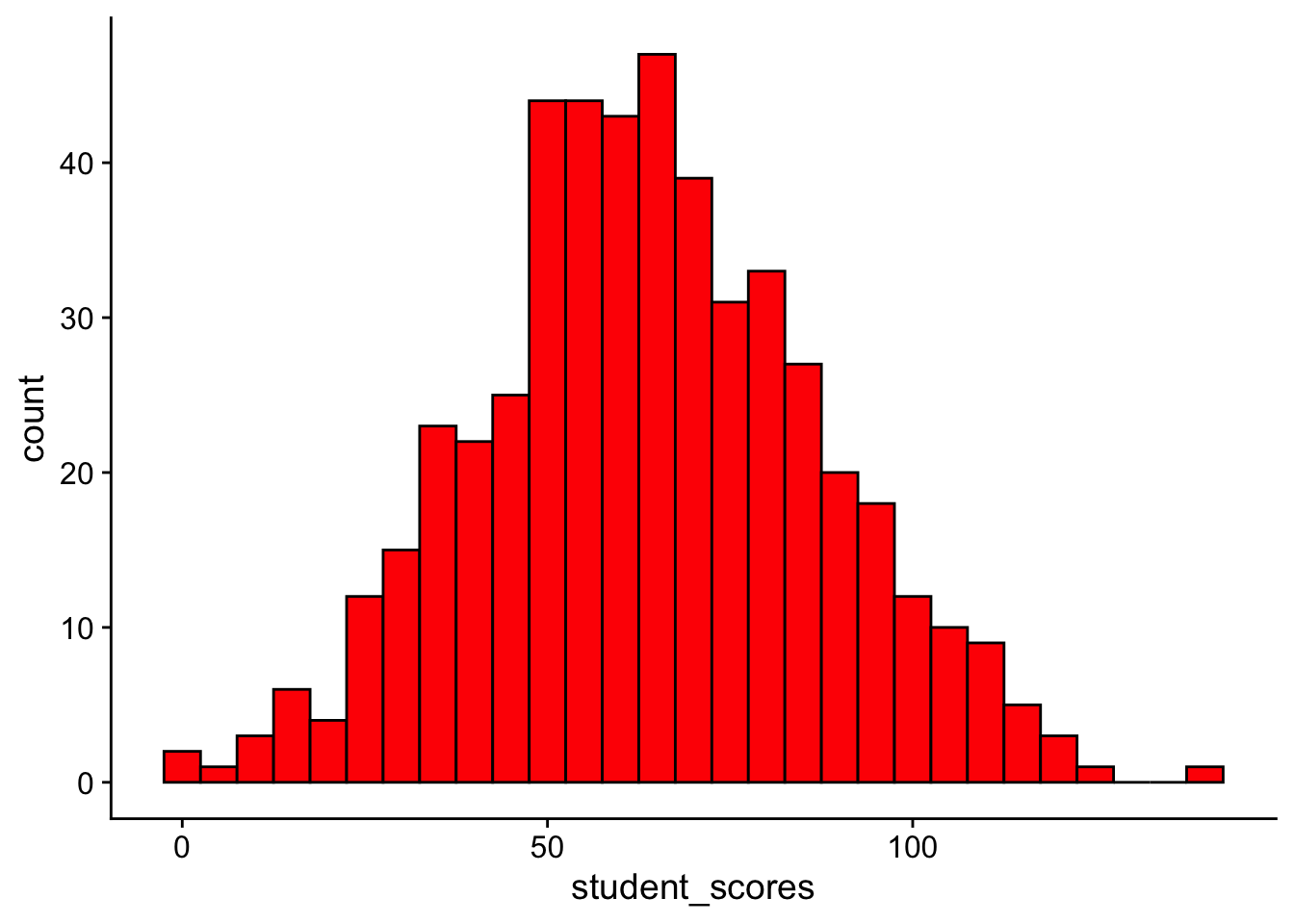

This will make much more sense next week, but for now we can define our means model formula as:

means_model <- lm(student_scores ~ 1, data = tjd_hs_data)

Now this is where the magic happens, we can take this model and submit it to a single function to get all the infomation we need about this model:

performance::check_model(means_model)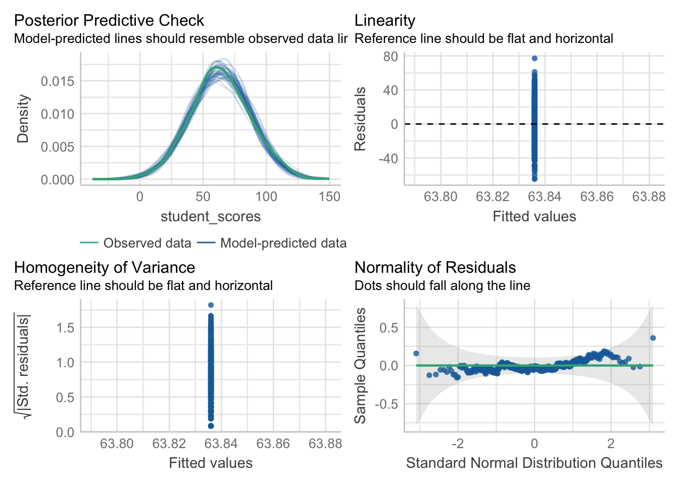

The perforance::check_model() function is designed to provide various model checks for regression models. The function provides easy access to various diagnostic plots and statistics. Its main use is for checking assumptions of linear regression models, such as linearity, independence, homoscedasticity, and normality of residuals. What I love most about this method is that the plots tell you exactly what to look for, aiding your visual inspection.

If you want run specific tests on the model residuals, this can be done as well.

To check for normality (using the Shapiro-Wilk’s method):

performance::check_normality(means_model)

OK: residuals appear as normally distributed (p = 0.832).

To check for heteroskedasticity / homogeneity of variance let’s consider our neighborhood income and home prices data.

two_hoods <- read_csv("http://tehrandav.is/courses/statistics/practice_datasets/two_hoods.csv")

Rows: 60 Columns: 2
── Column specification ────────────────────────────────────────────────────────
Delimiter: ","
chr (1): neighborhood
dbl (1): income

ℹ Use `spec()` to retrieve the full column specification for this data.
ℹ Specify the column types or set `show_col_types = FALSE` to quiet this message.

household_data <- read_csv("http://tehrandav.is/courses/statistics/practice_datasets/household_data.csv")

Rows: 200 Columns: 3
── Column specification ────────────────────────────────────────────────────────
Delimiter: ","
dbl (3): income, house_price, residuals

ℹ Use `spec()` to retrieve the full column specification for this data.
ℹ Specify the column types or set `show_col_types = FALSE` to quiet this message.

In both cases we’ll need first construct linear models of our relationship between our outcomes and predictors.

In the categorical case, we were investigating income as a function of neighborhood. Since our predictor is categorical we are testing for homogeneity. I’ll note for now this defaults to the Bartlet Test for homogeneity which is a slight variant of the Levene’s test. I’ll go into greater detail on this distinction when we get to ANOVA. (Levene’s Test and another test known as Fligner’s Test are also options here)

categorical_model <- lm(income~neighborhood, data = two_hoods)

performance::check_homogeneity(categorical_model, method = "bartlett")

Warning: Variances differ between groups (Bartlett Test, p = 0.005).

In the continuous case, we are investigaing house_prices as a function of income. Since our predictor is continuous, we are checking for heteroskedasticity using the Breush-Pagan Test:

continuous_model <- lm(house_price~income, household_data)
performance::check_heteroskedasticity(continuous_model)

Warning: Heteroscedasticity (non-constant error variance) detected (p = 0.005).

My recommendation is to use this package for all of your assumption tests this semester (and beyond)