pacman::p_load(tidyverse,
               car,
               cowplot,
psych)26 Independent samples t-test
This week we cover when and how to conduct a \(t-test\). We use a t-test to assess whether the observed difference between sample means is greater than would be predicted be chance. The Field text does a wonderful job of explaining t-tests conceptually so I will defer to those experts on matters of the underlying their statistical basis. Instead my goal this week is to walk through some examples on performing, interpreting, and reporting t-tests using R.
This walkthough assumes that the following packages are installed and loaded on your computer:
26.1 Things to consider before running the t-test
Before running a t.test there are a few practical and statistical considerations that must be taken. In fact, these considerations extend to every type of analysis that we will encounter for the remainder of the semester (and indeed the rest of your career) so it would be good to get in the habit of running through your checks. In what proceeds here I will walk step by step with how I condunct a t.test (while also highlighting certain decision points as they come up).
26.1.1 What is the nature of your sample data?
In other words where is the data coming from? Is it coming from a single sample of participants? Is it coming from multiple samples of the SAME participants? Is it coming from multiple groups of participants. This will not only determine what analysis you choose to run, but in also how you go about the business of preparing to run this analysis. Of course, truth be told this information should already be known before you even start collecting your data, which reinforces an important point, your central analyses should already be selected BEFORE you start collecting data! As you design your experiments you should do so in a way in which the statistics that you run are built into the design, not settled upon afterwards. This enables you to give the tests you perform the most power, as you are making predictions about the outcomes of your test a priori. This will become a major theme on the back half of the class, but best to introduce it now.
For this week, it will determine what test we will elect to perform. Let’s grab some sample data from an experiment from Aronson et al. (1999), original article here
26.1.2 Independent samples example
We run an independent samples t-test when we have reason to believe that the data in the two samples is NOT meaningfully related in any fashion. Consider this example regarding Joshua Aronson’s work on stereotype threat:
Joshua Aronson has done extensive work on what he refers to as “stereotype threat,” which refers to the fact that “members of stereotyped groups often feel extra pressure in situations where their behavior can confirm the negative reputation that their group lacks a valued ability” (Aronson, Lustina, Good, Keough, Steele, & Brown, 1998). This feeling of stereo- type threat is then hypothesized to affect performance, generally by lowering it from what it would have been had the individual not felt threatened. Considerable work has been done with ethnic groups who are stereotypically reputed to do poorly in some area, but Aronson et al. went a step further to ask if stereotype threat could actually lower the performance of white males—a group that is not normally associated with stereotype threat.
Aronson et al. (1999) used two independent groups of college students who were known to excel in mathematics, and for whom doing well in math was considered important. They assigned 11 students to a control group that was simply asked to complete a difficult mathematics exam. They assigned 12 students to a threat condition, in which they were told that Asian students typically did better than other students in math tests, and that the purpose of the exam was to help the experimenter to understand why this difference exists. Aronson reasoned that simply telling white students that Asians did better on math tests would arousal feelings of stereotype threat and diminish the students’ performance.
Here we have two mutually exclusive groups of white men, those that are controls and those under induced threat. Importantly we have no reason to believe that any one control man’s score is more closely tied to any individual experimental group counterpart than any others (we’ll return to this idea in a bit). In other words we have strong reason to accept that the two groups scores are Independent of one another (there goes that nasty Independence assumption again!)
26.1.3 Data cleaning and wrangling
Here is the data:
stereotype_data <-
  read_csv("http://tehrandav.is/courses/statistics/practice_datasets/stereotype_data.csv")
Rows: 22 Columns: 4
── Column specification ────────────────────────────────────────────────────────
Delimiter: ","
chr (2): ID, wID
dbl (2): Score, Group
ℹ Use `spec()` to retrieve the full column specification for this data.
ℹ Specify the column types or set `show_col_types = FALSE` to quiet this message.Now let’s take a look at the file structure:
stereotype_data# A tibble: 22 × 4
ID Score Group wID
<chr> <dbl> <dbl> <chr>
1 01 4 1 01
2 02 9 1 02
3 03 12 1 03
4 04 8 1 04
5 05 9 1 05
6 06 13 1 06
7 07 12 1 07
8 08 13 1 08
9 09 13 1 09
10 10 7 1 10
# ℹ 12 more rowsFor now, ignore the wID column, we’ll come back to that in the next walkthrough.
I like this example dataset as it gives is an opportunity to deal with a common issue in data cleaning. If you take a look at Group you see it’s either 1 or 2. In this case Group 1 are the control subjects and Group 2 are the threat subjects. Using numbers instead of names to identify levels of a factor is a convention from older methods and software. In more modern software you don’t need to do this sort of number coding (the software works this out in the background).
In fact, this convention can cause problems for us. Notice that R is treating the Group column as if it contains numerical data <dbl>. This is obviously not correct, these data are better described as nominal than numerical/continuous. Not correcting this mistake will have implications for our outcome. The testts will run, BUT the resulting outcome values will be incorrect (among other things this messes with the degrees of freedom for the model).
To change this, we can use the recode_factor() function from dplyr package in the tidyverse (https://dplyr.tidyverse.org/reference/recode.html). For what it’s worth there are several other ways to do this including a recode() function in car. See http://rprogramming.net/recode-data-in-r/ for examples.
Here I’m just going to mutate a new column, namedGroup column with the recoded names:
stereotype_data <- stereotype_data %>%
  mutate("namedGroup" = dplyr::recode_factor(Group,
                                            "1"="Control",
                                            "2"="Threat")
                            )
stereotype_data
# A tibble: 22 × 5
ID Score Group wID namedGroup
<chr> <dbl> <dbl> <chr> <fct>
1 01 4 1 01 Control
2 02 9 1 02 Control
3 03 12 1 03 Control
4 04 8 1 04 Control
5 05 9 1 05 Control
6 06 13 1 06 Control
7 07 12 1 07 Control
8 08 13 1 08 Control
9 09 13 1 09 Control
10 10 7 1 10 Control
# ℹ 12 more rows26.1.4 Checking our assumptions
Remember that you should always test to see if the data fit the assumptions of the test you intend to perform. In this case, we need to assess two things: homogeneity of variance and normality. Unfortunatley, the performance package does not work for the commonly used \(t\)-test functions. So, we’ll have to check our assumptions the old fashioned way. Here we will focus on the normailty assumption and the homogeneity assumption.
26.1.4.1 normality
No being able to use the performance package makes checking for normality a bit of a pain. Essentially, we need to split our two groups and run the requisite checks on each. I’ll show you how to do this step by step, before showing you how you can leverage some of the skills you picked up using DataCamp to make this a little less of a pain.
26.1.4.1.1 set-by-step (long way)
First let’s split our two groups
control_group <- stereotype_data %>% filter(namedGroup == "Control")
threat_group  <- stereotype_data %>% filter(namedGroup == "Threat")
And now to run the requisite assumption tests. Note that in this case I am running an Indepednent samples test, so I need to test the assumptions on each group separately.
First the Control Group:
We being with a visual qqPlot
car::qqPlot(control_group$Score)
[1] 1 11Now Shapiro-Wilkes
shapiro.test(control_group$Score)
    Shapiro-Wilk normality test

data:  control_group$Score
W = 0.89746, p-value = 0.1721
Both suggest to me that the control group data are normal.
Now moving onto the Threat Group
A visual qqPlot
car::qqPlot(threat_group$Score)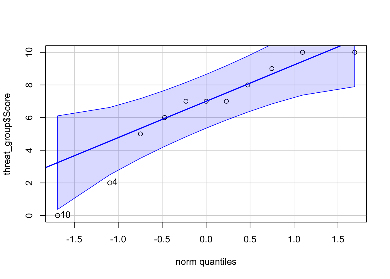
[1] 10 4Now Shapiro-Wilkes
shapiro.test(threat_group$Score)
    Shapiro-Wilk normality test

data:  threat_group$Score
W = 0.90317, p-value = 0.202
Looks like we are good here. No need to bring out the big guns (i.e. Bootstrapping)
26.1.4.1.2 short way using ggplot and tidy / dplyr
We can make use of some of the ggplot() skills and dplyr() verbs you learned in DataCamp to make this a little more efficient (although perhaps less read-able). Here is how I might create two seperate qqPlots()
pacman::p_load(qqplotr)

ggplot(stereotype_data, aes(sample = Score)) +
    stat_qq_point() +
    stat_qq_line() +
    stat_qq_band(alpha = 0.2) +
    theme_cowplot() +
    facet_wrap(~namedGroup)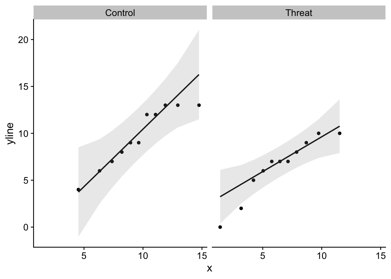
To execute the two Shapiro-Wilkes tests, we can:
stereotype_data %>%
    group_by(namedGroup) %>%
    select(Score) %>%
    summarise(
        shapiro = shapiro.test(Score)$p.value
    )
Adding missing grouping variables: `namedGroup`# A tibble: 2 × 2
namedGroup shapiro
<fct> <dbl>
1 Control 0.172
2 Threat 0.20226.1.4.2 Homogeniety of Variance
The Independence samples test assumes the variability of scores for the two groups is roughly homogeneous.
We can generate a simple table of our sample statistics using the psych::describeBy() function:
psych::describeBy(stereotype_data,
                  group = stereotype_data$namedGroup)
 Descriptive statistics by group
group: Control
            vars  n mean   sd median trimmed  mad min max range  skew kurtosis
ID*            1 11 6.00 3.32      6    6.00 4.45   1  11    10  0.00    -1.53
Score          2 11 9.64 3.17      9    9.89 4.45   4  13     9 -0.31    -1.48
Group          3 11 1.00 0.00      1    1.00 0.00   1   1     0   NaN      NaN
wID*           4 11 6.00 3.32      6    6.00 4.45   1  11    10  0.00    -1.53
namedGroup*    5 11 1.00 0.00      1    1.00 0.00   1   1     0   NaN      NaN
              se
ID*         1.00
Score       0.96
Group       0.00
wID*        1.00
namedGroup* 0.00
------------------------------------------------------------
group: Threat
            vars  n  mean   sd median trimmed  mad min max range  skew kurtosis
ID*            1 11 17.00 3.32     17   17.00 4.45  12  22    10  0.00    -1.53
Score          2 11  6.45 3.14      7    6.78 2.97   0  10    10 -0.73    -0.67
Group          3 11  2.00 0.00      2    2.00 0.00   2   2     0   NaN      NaN
wID*           4 11  6.00 3.32      6    6.00 4.45   1  11    10  0.00    -1.53
namedGroup*    5 11  2.00 0.00      2    2.00 0.00   2   2     0   NaN      NaN
              se
ID*         1.00
Score       0.95
Group       0.00
wID*        1.00
namedGroup* 0.00
or if we desire a cleaner table, we can pull out the values we are interested in ourselves:
stereotype_data %>%
    group_by(namedGroup) %>%
    summarise(
        n = n(),
        mean = mean(Score),
        sd = sd(Score),
        se = sd(Score)/sqrt(n()),
        var = sd(Score)^2
    )
# A tibble: 2 × 6
namedGroup n mean sd se var
<fct> <int> <dbl> <dbl> <dbl> <dbl>
1 Control 11 9.64 3.17 0.956 10.1
2 Threat 11 6.45 3.14 0.947 9.87In this table we see that our variances are roughly equal to one another. Let’s conduct a more stringent test using the leveneTest() from the car package:
# using long-format enter as a formula:
car::leveneTest(Score~namedGroup,
                data=stereotype_data,
                center="mean")
Levene's Test for Homogeneity of Variance (center = "mean")
Df F value Pr(>F)
group 1 0.2437 0.6269
20 You’ll note above I elected to mean center my samples. This is consistent with typical practice although “median” centering may be more robust.
car::leveneTest(Score~namedGroup,
                data=stereotype_data,
                center="median")
Levene's Test for Homogeneity of Variance (center = "median")
Df F value Pr(>F)
group 1 0.2907 0.5957
20 26.1.5 running the \(t\)-test
Given that my obtained Pr(>F), or p-value of Levene’s F-test, is greater than .05, I may elect to assume that my variances are equal. However, if you remained skeptical, there are adjustments that you may make. This includes adjusting the degrees of freedom according to Welch-Satterthwaite recommendation (see below). Recall later on that we are looking at our obtained \(t\) value with respect to the number of \(df\). This adjustment effectively reduces the \(df\) in turn making your test more conservative.
The Levene’s test failed to reject the null so I may proceed with my t.test assuming variances are equal. Note that we set paired=FALSE for independent sample tests:
t.test(data=stereotype_data, Score~namedGroup,
       paired=FALSE,
       var.equal=TRUE)
    Two Sample t-test

data:  Score by namedGroup
t = 2.364, df = 20, p-value = 0.02831
alternative hypothesis: true difference in means between group Control and group Threat is not equal to 0
95 percent confidence interval:
 0.3742243 5.9894120
sample estimates:
mean in group Control  mean in group Threat
             9.636364              6.454545
This output gives us the \(t\)-value (2.36), \(df\) (20) and \(p\)-value (.028). Based on this output I may conclude that the mean score in the Control group (9.636) is significantly greater than the Threat group (6.455).
Just as an example, let’s set var.equal to FALSE (afterall, technically the variances are not equal to one another) and see how this changes our results:
t.test(Score~namedGroup,
       data=stereotype_data,
       paired=FALSE,
       var.equal=FALSE)
    Welch Two Sample t-test

data:  Score by namedGroup
t = 2.364, df = 19.998, p-value = 0.02831
alternative hypothesis: true difference in means between group Control and group Threat is not equal to 0
95 percent confidence interval:
 0.3742093 5.9894270
sample estimates:
mean in group Control  mean in group Threat
             9.636364              6.454545
Comparing the outputs you see that in this case R has indicated that it has run the test with the Welsh correction. Note that this changes the \(df\) and consequently the resulting \(p\) value. That this change was negligible reinforces that the variances were very similar to one another. However in cases where they are not close to one another you may see dramatic changes in \(df\).
In R, the t.test() function sets var.equal=FALSE by default. Why you ask? Well, you can make the argument that the variances are ALWAYS unequal, its only a matter of degree. Assuming variances are unequal makes your test more conservative, meaning that if the test suggests that you should reject the null, you can be slightly more confident that you are not committing Type I error. At the same time, it could be argued that setting your var.equal=TRUE in this case (where the Levene test failed to reject the null) makes your test more powerful, and you should take advantage of that power to avoid Type II error.
In the next walkthrough we tackle how to conduct other types of tests. We’ll also provide examples of how to plot your data.