Embracing the Heteroskedasticity (or actually not)
Having wrestled with the beasts of independence and normality, let’s tackle another statistical assumption. Let’s dive into the realm of heteroskedasticity.
20.1 Hetero… what?
Heteroskedasticity… it’s mouthful, right? It’s a word that’s hard to say and even harder to spell. But it’s a word that’s important to understand. So let’s break it down.
Heteroskedasticity – or the lack of “homogeneity of variance” – simply means that the variability of a variable isn’t consistent across all levels of another variable. We typically refer to homogeneity of variance when we are testing with categorical predictors (like \(t\)-tests and ANOVA) and heteroskedasticity when considering continuous predictors (regression), but they are one in the same.
20.1.1 Categorical Example
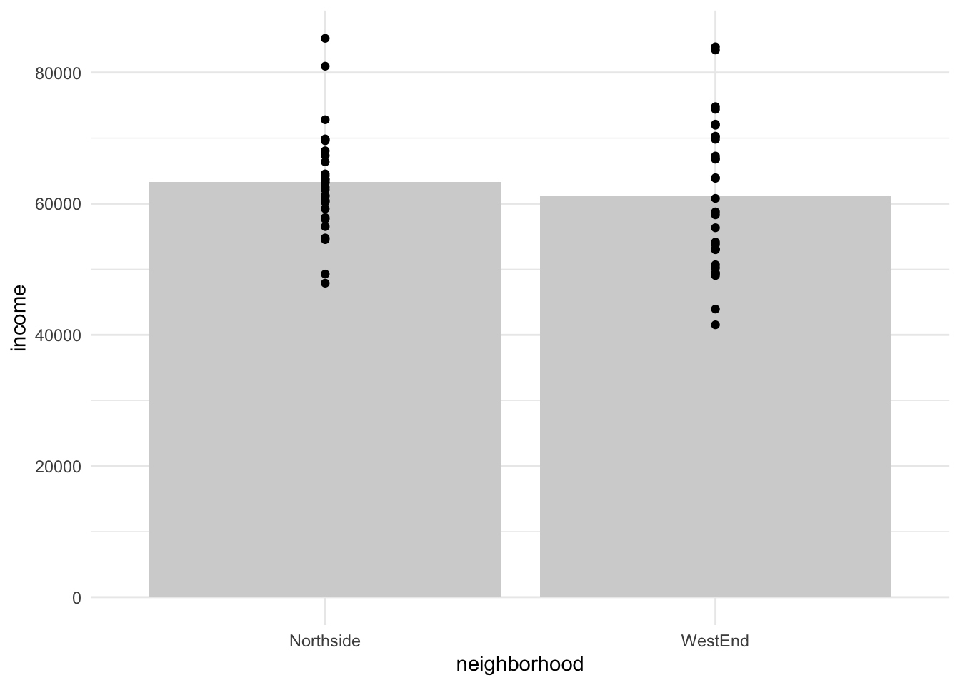
For example, let’s imagine that we are comparing the household incomes of two Cinci neighborhoods based on data from here
Warning: Using `size` aesthetic for lines was deprecated in ggplot2 3.4.0.
ℹ Please use `linewidth` instead.
As you can see in the plot above, even though the mean incomes for the neighborhoods are the same, the variances of the two neighborhoods are quite different. This reflects a wider dispersion of incomes in West End, where the mean is a consquence of a few high income households balancing against lower income households (gentrification, perhaps?). In Northside, the gap between households in our sample is not so great.
20.1.2 Continuous example
Suppose you’re analyzing data from West End, specifically looking at homeowners. One interesting aspect to consider is the connection between household income and the price of the homes they’ve purchased.
Common sense suggests that those with limited incomes might be restricted to homes within a certain price range, mainly because there’s a limit to how much house you can afford with a limited budget. However, as incomes increase, the range of choices also grows. A high-income household could afford a more expensive house, but they might also decide on a more modest home, allocating money elsewhere like investing or travel.
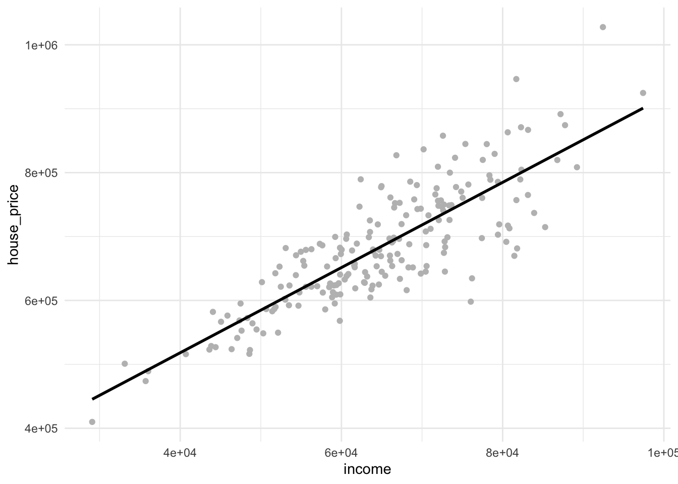
Given this, we might expect a greater variability in home prices among higher income households compared to those with lower incomes. Let’s take a look at some hypothetical data to illustrate this point.
set.seed(42)# Create a sample of 200 householdsn <-200income <-rnorm(n, mean =65000, sd =12000)# Generate house prices based on income, but introduce more variability for higher incomes and less for lower incomesbaseline_price <-230000+7* income# Adjust variability for higher and lower incomes# Here, we're using a fraction of the income as the standard deviation for the variabilityvariable_component <-rnorm(n, mean =0, sd = income * .8)house_price <- baseline_price + variable_component# Clamp house prices between 230K and 800Khousehold_data <-tibble(income, house_price)# Plotggplot(household_data, aes(x=income, y=house_price)) +geom_point(color="gray") +geom_smooth(method=lm, level =0.95, color="black", se =FALSE) +theme_minimal()
`geom_smooth()` using formula = 'y ~ x'
Examining the plot, you might observe a trend in the variability of home prices as incomes rise. This demonstrates the potential choices and variability middle and high-income earners have when purchasing homes in West End (compared to lower income earners).
20.2 Why is this an issue?
So what? Why does this matter? The answer lies in our second plot. Looking at the plot again, what stands out?
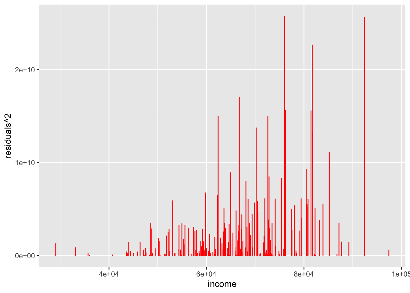
If you guessed “the predictive model tends to perform worse for middle income earners” then you’d be correct!. To really hammer this home let’s create a plot of the model error (residuals) as a function of income.
model <-lm(house_price~income, household_data)model_residuals <-residuals(model)household_data <- household_data %>%mutate(residuals = model_residuals)ggplot(household_data, aes(x = income, y = residuals^2)) +geom_col(color ="red")
Ideally we’d like these residuals to be consistent across the entire range of incomes.
20.3 Testing for heteroskedasticity
More often than not, you’ll be testing for heteroskedasticity in the context of a model. Using our two examples above we can build two very simple linear models for now that we can revisit in upcoming weeks. In the categorical predictors case, we had two neighborhoods that we were comparing for income. As simple model here would be to look at our outcome variable, income as a function of our predictor(s), neighborhood. In R the ~ symbol is literally interpreted as “is a function of”, so we can write this relationship as: income ~ neighborhood
We can define this simple linear model as so:
categorical_model <-lm(formula = income ~ neighborhood, data = two_hoods)
To test for homogeneity of variance with categorial predictors we use Levene’s Test. A basic version of this test can be performed using car::leveneTest (note that car is installed on base R so you should not need to install it).
car::leveneTest(categorical_model)
Warning in leveneTest.default(y = y, group = group, ...): group coerced to
factor.
Levene's Test for Homogeneity of Variance (center = median)
      Df F value   Pr(>F)
group  1  7.3826 0.008667 **
      58
---
Signif. codes:  0 '***' 0.001 '**' 0.01 '*' 0.05 '.' 0.1 ' ' 1
The null hypothesis of the leveneTest is that the groups’ variances are homogeneous. Thus, a p < than .05 is seen as sufficient evidence to reject the null.
For continuous predictors, we can use the Breusch-Pagan Test. This test is not available in base R but can be found in the olsrr package. Let’s consider our continuous predictor example predicting house price as a function of houldhold income, or house_price~income:
 Breusch Pagan Test for Heteroskedasticity
 -----------------------------------------
 Ho: the variance is constant
 Ha: the variance is not constant

                 Data
 ---------------------------------------
 Response : house_price
 Variables: fitted values of house_price

         Test Summary
 ------------------------------
 DF            =    1
 Chi2          =    32.04486
 Prob > Chi2   =    1.50653e-08
As with the Levene’s Test, the null hypothesis here is that the variance is homogeneous, or rather NOT heteroskedastic. Therefore a reported p-value (here evaluated along the \(\chi^2\) distribution (Chi2) that is less than .05 means that the model has violated this assumption.