18.1 Thinking about probability and assumptions of our data.
In this walkthrough, we dive a little bit further into probability and how it directly factors into our assessments on important aspects of our data. This will lead into our future discussions regarding statistics tests and inference making.
For the next few weeks, these two critical assumptions about the nature of our observed data will be paramount:
that the data (its distribution) is randomly obtained from a normal population.
that our measures of the data (including both the tools we use to get our measures and the resulting descriptions of the data) are independent of one another.
We’ve spent some time at length with Assumption #1 in the previous two walkthroughs (15 and 16) noting a few things about the normal distribution:
It was long considered to be a statistical representation of all naturally occurring phenomena (assuming random chance) although now we appreciate it as more the exception than the rule—many phenomena we are interested do not abide the normal distribution.
Even if (1) is the case, the Central Limit Theorem saves us, demonstrating that with sufficiently large sample sizes, the sampling distribution of the sample mean will approximate a normal distribution, regardless of the distribution of the underlying data. This is important because many classical statistical methods, like the t-test or ANOVA, are based on the assumption that the sampling distribution of the statistic (often the mean) is normally distributed. Therefore, even if our raw data isn’t normal, the Central Limit Theorem ensures that we can still employ these techniques with reasonable confidence when our sample sizes are large (Walkthough 15).
The central reason for its importance is that the probabilities of specific outcomes related to the normal distribution are known (Walkthrough 16). Having said that there other well known distributions, including the binomial distribution (which we’ll play with a little bit today).
In this walkthrough I want to shift briefly to Assumption #2, the independence of measures. Let’s discuss the deep implications of this assumption, some “laws” of probability that can be derived from this assumption, and what it means to violate indepence (good and bad).
I’ll start with an example that I use in my Perception course:
Say I step on a scale and it says that I’m 180 lbs. I then walk over to a stadiometer and get my height measured and it tells me I’m 71 inches tall. Right after this I return to the original scale. If the measurement of my weight and height were independent of one another, then the scale should again read 180 lbs. However, if in some stange reality, the act of measuring my height somehow changes the measurement of my weight, then all bets are off—the second time on the scale it could say I’m 250 lbs, 85 lbs, who knows.
One of the lessons of quantum mechanics (see Stern-Gerlach experiments is that we do live in that strange reality—at least at the quantum level. Most of you have probably encountered the uncertainty principle which is a physical manifestation of this issue. More pertinent for us consider the following:
We have a theory that adults with children are less likely to smoke than adults without children, due to concerns about secondhand smoke exposure, setting a good example, and general health concerns. Our null hypothesis is that adults with children are no less likely to smoke than adults without children.
Here, individuals are being assessed based on:
The smoking behavior measurement (do you smoke, yes or no?)
The parenthood measurement (do you have a child, yes or no?).
If these two measures are independent of one another, then the smoking behavior should not influence the parenthood measurement and vice versa. If they are not independent, it suggests there might be a relationship between being a parent and one’s likelihood to smoke. This doesn’t mean that starting or quitting smoking can instantly affect your parental status (YIKES), but it does suggest that having children might influence one’s decision about smoking.
Hopefully from this example, you now see the relationship between the null and research (alternative) hypotheses. Our null hypothesis was that smoking behavior and parenthood were unrelated, meaning they were independent. The research hypothesis is structured in such a way that it assumes a violation of the null, in this case, a violation of the independence assumption. In testing our hypotheses, we will be examining whether the evidence supports such a violation. The evidence in this case would be a change in the probability of being a smoker if one was also a parent. To get a feel for how we evaluate this, we need to delve into the laws of probability.
18.1.1 The laws of probability
There are several central laws of probability that, in our context, help us understand and quantify the likelihood of observing certain data given our null hypothesis. These laws form the backbone of hypothesis testing. For our purposes, let’s consider a sample of 100 people that have been identified by whether or not they are parents AND whether or not they are smokers.
For our purposes, we can consider the simple probability of being a parent as \(P(A)\) and the simple probability of being a smoker as \(P(B)\). Using this notation, we can make several claims:
Joint Probability: The Multiplication Rule states that the joint probability of two independent events happening together is the product of their individual probabilities. For instance, if the probability of being a parent \(P(A)\) and the probability of being a smoker \(P(B)\) were independent, then the probability of both being a parent and being a smoker \(P(A \text{ and } B)\) would simply be \(P(A) \times P(B)\).
Addition Rule: If two events are mutually exclusive (they cannot both happen at the same time), then the probability of either event happening is the sum of their individual probabilities: \[
P(A \text{ or } B) = P(A) + P(B)
\] However, if the events are not mutually exclusive (they can occur simultaneously), the probability of either event happening is: \[
P(A \text{ or } B) = P(A) + P(B) - P(A \text{ and } B)
\]
Conditional Probability: This is the probability of an event happening given that another event has already occurred. For instance, \(P(B|A)\) represents the probability of being a smoker given that one is a parent. If \(P(B|A)\) differs from \(P(B)\), then it suggests that being a parent influences smoking behavior.
In the context of our study, the null hypothesis asserts that the probability of being a smoker, given one is a parent \(P(B|A)\), is the same as the overall probability of being a smoker \(P(B)\). The alternative hypothesis suggests a difference, implying that parenthood has an effect on smoking behavior.
By using a contingency table, we can compute observed and expected frequencies for each combination of our two categories: smokers/non-smokers and parents/non-parents. If our observed frequencies significantly deviate from what we would expect under the null hypothesis (using the laws of probability), we might reject the null in favor of the alternative.
Rows: 100 Columns: 2
── Column specification ────────────────────────────────────────────────────────
Delimiter: ","
chr (2): Parent, Smoker

ℹ Use `spec()` to retrieve the full column specification for this data.
ℹ Specify the column types or set `show_col_types = FALSE` to quiet this message.
And let’s look at the outcomes:
parenthood_smoking_data %>%count(Parent, Smoker)
# A tibble: 4 × 3
  Parent Smoker     n
  <chr>  <chr>  <int>
1 No     No        36
2 No     Yes        7
3 Yes    No        40
4 Yes    Yes       17
From here we can what we know from our Rules for Probability. In particular, if Smoking and Parenthood are independent, then our observed probability of being “Parent who Smokes” should be roughly equal to the joint probability of being a Smoker, \(P(\text{Smoker})\), and a Parent, \((P\text{Parent})\). Looking at the table above the probability of being a smoking parent (Parent: Y; Smoker: Y) is .17. The Probability of being a parent overall is .57 (40 +17) and the probability of being a smoker is .24 (7 + 17). Thus, using the multiplication rule: \[
P(\text{Smoker}) \times P(\text{Parent}) = .57 \times .24 ≈ .137
\]
Meaning with true independence we should expect about 14 smoking parents. We observed 17. Is this difference big enough? We’ll come back to that the end of this section. For now, let’s talk about my sneaker-game.
18.2 Harper and Sadie’s daddy needs a new pair of Jordans
While we are primarily dealing with continuous data, I find that intuitions about probability are best made using examples from discrete outcomes (see Cohen Chapter 19 if you want to look ahead at the Binomial Distribution; if not we’ll get there at the end of the semester). The classical examples are rolling die and flipping a coin. So..
Let’s make a wager. I’ll let you flip a single coin 10 times, and if you get 6 or more heads I’ll give you $250. If not, you have to give me $250. Should you take this bet? To answer this question you’ll want to assess the likelihood of getting an observed outcome, in this case \(Heads \geq 6\), provided a sample size (10).
We assume that the likelihood of getting Heads on any single flip is .5, (assuming that the coin is far and not a cheat). This is our expected probability. We also assume that the coin flips are independent of one another, that is any single flip does not influence or change the likelihood of an outcome on subsequent flips. Given this assumption we can apply the joint probability to calculate expected outomes of multiple events. For example if we flip a coin twice the probability of both flips landing heads is \(.5 \times .5 = .25\)
*In light of our discussion in the opening section, I hope you see that depending on the outcome, it may cause us to re-evaluate these two assumptions—fair coin, independent flips.
For now, let’s assume that both are indeed true and that I’m not a cheat.
18.2.1 How many heads would we get if we flipped a fair coin 10 times?
In class we noted that with a known sample space and a known sample size we can calculate the expected outcome. In this case our sample space is {Heads, Tails} and our sample size is 10 (flips). The probability of observing a Heads in our sample space is .5. Therefore:
Of course, reality does not often abide our expectations, and given what we know about sampling error you’re more likely to not get exactly 5 flips than you are. So, what we’re really interested in is what is the likelihood of our expectation, and fortunately for us, over the long-run independent/random outcomes can be predicted probabilistically. There are several ways to address this in R.
18.2.1.1 Simulation method
The first method involves running a large number of simulations and assessing the probability based upon the outcomes. To run a single simulation, you can use the rbinom() function. Below I am running a simulation of 1 coin (n), with a sample size of ten flips (size), and a known (or really assumed) probability of .5 (prob).
# set our seeds to get the same numbers:set.seed(1)# n = number of coins# size = number of flips# prob(ability)rbinom(n =1,size =10,prob = .5)
[1] 4
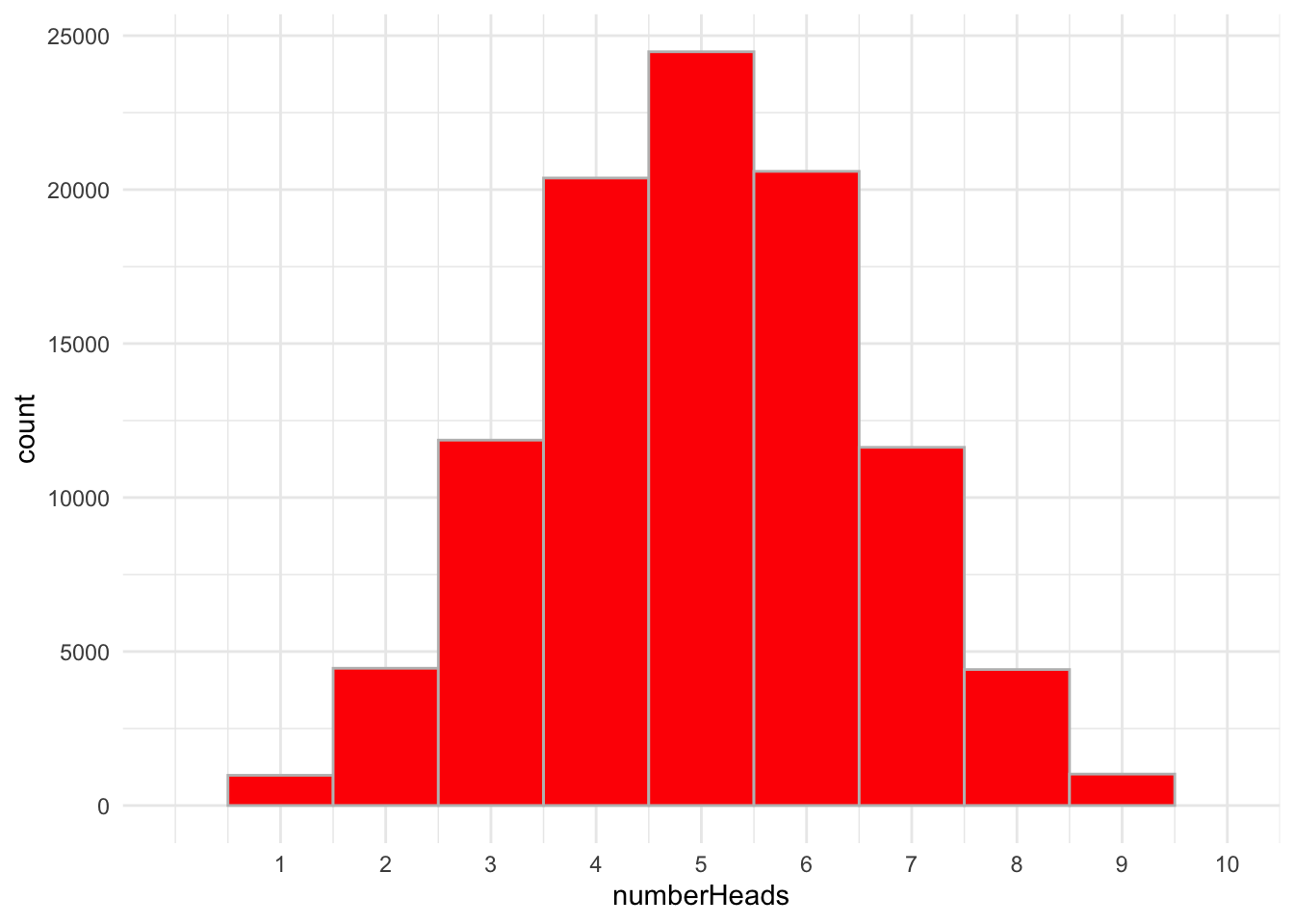
In this simulation you got 4 flips and I’m off to cop a new pair of retro Air Jordans with your money… or I suppose if I’m being sensible, you’ve paid for this week’s daycare. In any event, you lost. But we know that not much can be learned about the likelihood of an outcome with a sample size of 1. Let’s try running this scenario using a simulation of 100K coins.
To run this simulation, you modify the rbinom() call:
As you can see in the plot above, we get exactly 5 heads a little less than 25K out of 100K, or about 25% of the time. That’s the eyeball test, How might we go about obtaining the exact probabilities from this simulation? We can take advantage of logical statements. Logicals produce outputs that are either TRUE or FALSE. More, and this is terribly useful for us, R also reads those TRUE or FALSE outcomes as 1 or 0 where TRUE=1 and FALSE=0. Take the following vector for example:
What this means is that you can get info about the number of TRUEs by performing mathematical operations on this vector. For example, above you see that there are 4 TRUEs out of 10 possible. That means that we get TRUE 40% of the time. We can obtain this probability in R using the mean() function. How? Remember that the mean is the sum of scores divided by the number of scores. In this case the sum is 4; the number of scores is 10; and 4/10 is .40.
Returning to our simulation of 100K samples, numberHeads, we can do the following to get the probability of 5 (see Demos, Ch. 3 on logicals for explanation of operators like ==):
mean(numberHeads==5)
[1] 0.24477
So the probability of getting exactly 5 heads is 0.245.
Returning to our wager, based on our simulation what’s the probability of getting 6 or more heads?
mean(numberHeads>=6)
[1] 0.37743
About 38%. You probably shouldn’t take my bet.
18.2.1.2 Non-simulation method
Simulations are useful for helping us visualize our scenarios and use pseudo real data to test our underlying assumptions. But most times you just want the answer… in fact often that will suffice because as I mentioned, in most normal circumstances the probabilities have already been worked out. How can we get the results above without simulating 100K coins? By using two functions in R that belong to the same family as rbinom(): dbinom() and pbinom().
dbinom() returns the exact probability of an outcome, provided a generated probability density function. It takes in arguments related to the number of successful outcomes (x), the sample size (size) and the independent probability of a successful outcome (prob).
So the probability of 5 Heads (successes) on 10 flips with a fair coin would be entered:
dbinom(x =5,size =10,prob = .5)
[1] 0.2460938
We see that this value is pretty close to our simulated outcome, confirming that the simulation was indeed correct, if not entirely necessary.
We can also use this function to build a table for the individual probabilities of all possible outcomes. To see how, first lets consider the space of possible outcomes in this scenario. At one extreme, I could flip a coin 10 times and get no Heads. At the other I could get all Heads. So the set of possible outcomes can be express as a sequence from 0 to 10. Recall that you can create such a sequence using the : operator:
0:10
[1] 0 1 2 3 4 5 6 7 8 9 10
With this in mind you can modify the previous code like so:
The output gives be the resulting probabilities in order from 0 Heads to 10 Heads.
Let’s create a table to make this easier to digest. First I’m going to create a vector of numberHeads to show all possibilities from 0 to 10. Second, I will run dbinom() as above to test each possibility, saving that to a vector probHead. Finally I will combine the two into a data frame called probTable:
# 1. range of possibilitiesnumberHeads <-0:10# 2. prob of outcomeprobHead <-dbinom(x = numberHeads,size =10,prob = .5)# 3. combine to data frameprobTable <-tibble(numberHeads,probHead)# 4. Show the data frame (table)show(probTable)
Congrats you’ve just created a Binomial Distribution Probability Table for this scenario. We’re a bit ahead of the game here as we deal with the Binomial Distribution at the end of the semester, but the general intuitions hold regarding the Normal Distribution as well.
Returning to our wager of 6 or more heads, we would use pbinom(). pbinom() returns probabilities according to the cumulative density function, where the output is the likelihood of obtaining that score or less. Note that pbinom() takes similar arguments to dbinom() but asks for q instead of x. For our purposes q and x are the same thing… number of outcomes.
So for example the probability of obtaining 5 or less Heads provided our scenario may be calculated:
pbinom(q =5,size =10,prob = .5)
[1] 0.6230469
Given what we know about the Compliment Law, we can compute the probability of 6 or more Heads as:
1-pbinom(q =5,size =10,prob = .5)
[1] 0.3769531
which again matches with our simulation.
18.3 Changing the parameters
So obviously if the coin is a fair coin, you shouldn’t take the bet. Let’s imagine that we kept the same wager, but to entice you to bet, I tell you that this coin lands on Heads 65% of the time? Should you take the bet?
To test this new scenario all you need to do is change the probability parameter. Let’s just skip the simulations and just assess using dbinom() and pbinom().
18.3.1 Constructing a table of outcome probabilities:
As before we’ll use dbinom() to create a table, simply modifying the prob argument to .65:
# 1. range of possibilitiesnumberHeads <-0:10# 2. prob of outcomeprobHead <-dbinom(x = numberHeads,size =10,prob = .65)# 3. combine to data frameprobTable <-tibble(numberHeads,probHead)# 4. Show the data frame (table)show(probTable)
Ahhh… the odds are ever so slightly in your favor.
What if we changed the bet: you get 60 Heads out of 100 flips?
1-pbinom(q =60,size =100,prob = .65)
[1] 0.827585
Yea, you should really take that bet! Fortunately for me, I wasn’t born yesterday.
How about 12 out of 20?
1-pbinom(q =12,size =20,prob = .65)
[1] 0.6010266
Nope, I’m not taking that bet either. Does 3 out of 5 interest you?
1-pbinom(q =3,size =5,prob = .65)
[1] 0.428415
18.4 Catching a cheat
OK. Last scenario. Let’s imagine that I am not a total sucker, and we reach a compromise on “30 or more Heads out of 50 flips”. You run to your computer and calculate your odds and like your chances (maybe I am a sucker)!
1-pbinom(q =30,size =50,prob = .65)
[1] 0.7264363
You flip 50 times but only get 27 heads. Astounded, because those odds really were in your favor, you label me a liar and a thief. Are you justified in doing so? This scenario essentially captures our discussion at the outset, how far of a deviation warrants us being skeptical that our original assumptions were true. In this case the original assumptions were that 1. each coin flip is independent and 2. the independent probability of getting a Heads is 0.65. We typically set our threshold at \(p<.05\), which remember for a two tailed test means that we are on the lookout of extreme values with a \(p<.025\).
So essentially we are asking if the probability of obtaining exactly 27 Heads given this scenario is less than 2.5%:
dbinom(x =27,size =50,prob = .65)
[1] 0.03132011
You Madam/Sir have besmirched my honor!
OK, well is 27 isn’t enough, then how low (or high) do you need to go to pass the critical threshold? To answer this we need to construct a table of probabilities:
# 1. range of possibilitiesnumberHeads <-0:50# 2. prob of outcomeprobHead <-dbinom(x = numberHeads,size =50,prob = .65)# 3. combine to data frameprobTable <-tibble(numberHeads,probHead)# 4. Show the data frame (table)show(probTable)
One could visually inspect the entire table noting which outcomes have a corresponding probability less than .025. But the whole point of learning R is to let it do the heavy lift for you. In this case you can ask R:
“Hey, R. Which outcomes in have a probability less than .025”
or more exactly:
“Which rows in my data frame have a probHead less than .025”
Note that in the above example I’m piping into DT::datatable to create the interactive table on this page. This is a cool function for displaying in hmtl rendered outputs, BUT depending on your environment it may not show up in your actual notebook.
From this table we see any number 26 or less would be suspect. So, if you got 1 less head, then you can call me a cheat. Conversely if you managed to get 39 heads or above, I might have reason to believe that you are somehow gaming me.
18.5 A final word on independence
In this walkthrough, we delved deep into the concept of the Independence Assumption. This assumption isn’t just a minor detail; it’s foundational to the entire process of Null Hypothesis Significance Testing (NHST). At its core, the Independence Assumption asserts that observations within a dataset are not related or dependent on one another, unless accounted for within the model.
One might wonder why so much emphasis is placed on this assumption. The reason is tied to the fundamental principles of inferential statistics. When we’re testing hypotheses, we’re trying to make broad generalizations about populations based on samples. For these generalizations to hold true, each observation in our sample needs to represent an independent piece of information about the population. If our observations are dependent on each other, our sample could be biased, leading to flawed conclusions.
This brings us to the term “independent variables.” The very name emphasizes our statistical hope and dreams and aspiration: we desire variables that are not influenced by other factors we’re examining in a study. This is particularly critical in experimental designs where we manipulate these independent variables to ascertain their effect on dependent variables. In an ideal scenario, when we manipulate an independent variable, any observed changes in the dependent variable can be confidently attributed to our manipulation, rather than some unaccounted-for external factor. This only holds if our independent variables are indeed “independent” and are not intertwined with other unmeasured variables in the system.
In essence, the concept of “independence” permeates every facet of statistical testing. When we make an assumption of independence, we’re asserting that our data points, variables, and resulting conclusions stand on their own, free from undue influence or bias. This foundational assumption is what allows us to draw robust, meaningful conclusions from our data.
However as my grad advisor said to a student who used the word “hope” when responding to a question during his thesis defense, “All of your hopes and your dreams will not not get you through this defense” (It was said pretty tongue and cheek, don’t worry said student actual laughed a bit and then settled kicked butt; FWIW said student was not me). True story, when dealing with something as complex as people we can rarely isolate any variable independent of a whole host of others.
That said, for now let’s just stick our heads back into the ontological sand. But before we leave…
18.6 Getting a little ahead of ourselves
At the beginning, we delved into a scenario examining the relationship between parenthood and smoking, using it as a backdrop to contrast observed outcomes with predictions based on the assumption of independence. I then pivoted—hopefully not too abruptly—to discuss coin flips, as they present a more straightforward context for these comparisons. However, I left you hanging with this thought:
If we assume true independence between parenthood and smoking, we’d expect to see around 14 smoking parents. But, we observed 17. Is this deviation significant?
While we could apply the logic from the coin-flip example to determine the significance of this discrepancy, there’s a more tailored approach at our disposal: the Chi-square contingency analysis.
This method, often referred to simply as “Chi-square” or \(\chi^2\), provides a robust tool for assessing the independence of categorical variables. It compares the observed frequencies of categories with the expected frequencies under the assumption of independence. In our case, it can help answer the question—just how significant is the difference between the expected 14 smoking parents and the observed 17? Through Chi-square, we can evaluate if such a difference could have arisen by chance alone or if there’s a more substantial pattern at play.
To employ \(\chi^2\) we can use the gmodels package and its CrossTable() function. We can simply create a contingency table as we did above and pipe it into gmodels::CrossTable() settingexpected = TRUE`.
   Cell Contents
|-------------------------|
|                       N |
|              Expected N |
| Chi-square contribution |
|           N / Row Total |
|           N / Col Total |
|         N / Table Total |
|-------------------------|


Total Observations in Table:  100


             | Smoker
      Parent |        No |       Yes | Row Total |
-------------|-----------|-----------|-----------|
          No |        36 |         7 |        43 |
             |    32.680 |    10.320 |           |
             |     0.337 |     1.068 |           |
             |     0.837 |     0.163 |     0.430 |
             |     0.474 |     0.292 |           |
             |     0.360 |     0.070 |           |
-------------|-----------|-----------|-----------|
         Yes |        40 |        17 |        57 |
             |    43.320 |    13.680 |           |
             |     0.254 |     0.806 |           |
             |     0.702 |     0.298 |     0.570 |
             |     0.526 |     0.708 |           |
             |     0.400 |     0.170 |           |
-------------|-----------|-----------|-----------|
Column Total |        76 |        24 |       100 |
             |     0.760 |     0.240 |           |
-------------|-----------|-----------|-----------|


Statistics for All Table Factors


Pearson's Chi-squared test
------------------------------------------------------------
Chi^2 =  2.465517     d.f. =  1     p =  0.1163694

Pearson's Chi-squared test with Yates' continuity correction
------------------------------------------------------------
Chi^2 =  1.778812     d.f. =  1     p =  0.1822953
The outcome test “Pearson’s Chi-squared test” in this case has a \(p\) = .116, suggesting we don’t have enough evidence to assume a relationship between Parenthood and Smoking—i.e., independence is not violated in this data.
Rows: 100 Columns: 2
── Column specification ────────────────────────────────────────────────────────
Delimiter: ","
chr (2): Parent, Smoker

ℹ Use `spec()` to retrieve the full column specification for this data.
ℹ Specify the column types or set `show_col_types = FALSE` to quiet this message.
And now to test these data. Here is the resulting contingency table:
   Cell Contents
|-------------------------|
|                       N |
|              Expected N |
| Chi-square contribution |
|           N / Row Total |
|           N / Col Total |
|         N / Table Total |
|-------------------------|


Total Observations in Table:  100


             | Smoker
      Parent |        No |       Yes | Row Total |
-------------|-----------|-----------|-----------|
          No |        23 |        20 |        43 |
             |    29.240 |    13.760 |           |
             |     1.332 |     2.830 |           |
             |     0.535 |     0.465 |     0.430 |
             |     0.338 |     0.625 |           |
             |     0.230 |     0.200 |           |
-------------|-----------|-----------|-----------|
         Yes |        45 |        12 |        57 |
             |    38.760 |    18.240 |           |
             |     1.005 |     2.135 |           |
             |     0.789 |     0.211 |     0.570 |
             |     0.662 |     0.375 |           |
             |     0.450 |     0.120 |           |
-------------|-----------|-----------|-----------|
Column Total |        68 |        32 |       100 |
             |     0.680 |     0.320 |           |
-------------|-----------|-----------|-----------|


Statistics for All Table Factors


Pearson's Chi-squared test
------------------------------------------------------------
Chi^2 =  7.300742     d.f. =  1     p =  0.006892616

Pearson's Chi-squared test with Yates' continuity correction
------------------------------------------------------------
Chi^2 =  6.177626     d.f. =  1     p =  0.01293758
Going off of this dataset we would assume a relationship between variables.
In conclusion, the \(\chi^2\) test is an essential tool in statistical analysis. It offers a way to evaluate the goodness of fit, essentially checking if our model’s predictions are in tune with what we observe in the real world. Beyond that, it serves as a mechanism to test for the independence of categorical variables, as illustrated with our parenthood and smoking example. Looking ahead, we’ll see that the \(\chi^2\) test isn’t limited to just these applications. It can be harnessed to compare different models, something we’ll dive deeper into next semester. Additionally, its principles can be adapted to assess inter-rater reliability, ensuring that multiple evaluators are consistent in their assessments. All in all, the Chi-square test is a versatile and indispensable part of statistical research. See you in our next discussion!