pacman::p_load(psych, tidyverse, sjstats)17 Sampling distributions and parameter estimates
Up to this point in class, we’ve laid out the logic of the sampling distribution (of means), the difference distribution (of means) and the null distribution (of means). In the workshop we made it as far as simulating the sampling distribution and using it to obtain important measures and to generate the distribution of means. Here I’m going to extend that work to show how to get both the difference distribution and the null distribution. This involves minor tweaks of what was done in class.
Please follow along by entering the commands into your own console. First let’s load in the appropriate packages for this week:
17.1 Population v. sample parameters
To begin let’s again start off with a population. For the sake of example, let’s imagine that this population represents the obtained State Achievement Scores of students in Tehran J. Davis High School (apparently I’m feeling myself) that were taught using a standard curriculum. The 500 students in this population have a mean score of 28.2 with a standard deviation of 11.7. Note that this mean and sd are FACTS… they are true values that exist independent of my measure. Also note that in real work, these truths about the population are rarely known. FWIW, you can read up, and see how these values might compate to Ohio State averages on page 2, here.
We can create a simulated population using the following chunk of code; note that anytime you are generating “random” distributions or “random” sampling in R you’ll need to input the set.seed(2023) command where I do to ensure that you get the same numbers I do.
First, let’s create a distribution of student
set.seed(2023)
student_scores <- rnorm(n = 500, mean = 28.2, sd = 11.7)
And next let’s combine this distribution with a list of student IDs (randomly generated) to create our data frame:
student_id <- sample(x = 100000:999999, size = 500)This is a bit of a Level-Up, so I’ll explain what we did here.
sample(): The sample() function in R is used to randomly sample a specified number of values from a given set of values. It can be used to generate random samples of data.100000:99999: This is the first argument to the sample() function and defines the set of values from which the random sample will be taken. In this case, it’s a range from 100,000 to 999,999.500: This is the second argument to the sample() function, indicating that you want to sample 500 values from the set of values specified in the next argument.
So, when you run this code, it will generate a random sample of 500 numbers, and each of these numbers will be within the range of 100,000 to 999,999. Note that we’re not guarenteed that each of the IDs will be unique (there is a small chance of duplicates), but to do so would require a little bit of tinkering that not useful for this example.
Now we can combine our student_id and our student_scores into single data frame tjd_hs_data:
tjd_hs_data <- tibble(student_id, student_scores)
head(tjd_hs_data)
# A tibble: 6 × 2
student_id student_scores
<int> <dbl>
1 236248 27.2
2 291594 16.7
3 436433 6.26
4 897223 26.0
5 283329 20.8
6 992358 41.0 When we take a look at what the above simulation generates, we see that the obtained values are sightly different than requested (it is random after all). BUT AGAIN, for the purposes of example these are still the facts of the population.
mean(tjd_hs_data$student_scores)[1] 28.25608sjstats::sd_pop(tjd_hs_data$student_scores)[1] 11.44974Wait… what’s that sjstats::sd_pop() mess?!?!?
To understand this we need to revisit our equation for calculating the standard deviation from a few week’s back. To remind ourselves, we said that we can calculate the standand deviation of a distribution of scores as: \[ SD = \sqrt{\frac{\sum(X-\bar{X})^2}{N - 1}} \]
where \(X\) is the score, \(\bar{X}\) is the mean of the scores, and \(N\) is the number of scores. This is the equation for the sample standard deviation. However, the population standard deviation is calculated as:
\[ \sigma = \sqrt{\frac{\sum(X-\mu)^2}{N}} \]
where \(\sigma\) is the population standard deviation, \(X\) represents an individual score, \(\mu\) is the population mean, and \(N\) denotes the total number of scores in the population.
Notice the differences: for the sample standard deviation, we divide by \(N-1\) (a practice known as Bessel’s correction), while for the population standard deviation, we simply divide by \(N\). The subtraction of 1 in the sample formula accounts for the degrees of freedom and tends to give a more unbiased estimate of the population standard deviation when we are working with a sample. The previous sentence introduced two important ideas: degrees of freedom and biased v. unbiased estimates. We’ll cover the latter in a few moments, but for now let’s talk a bit about degrees of freedom.
17.2 Degrees of Freedom
A long time ago and not so far way, I rememer being told that March Madness (the College Basketball tournament for those outside of the know) took 63 games to determine a winner. This was long ago when the tournament only had 64 teams (dating myself here a bit). I remember at first thinking “that can’t be right, that’s seems a little high”. But, upon further reflection, the logic became clear: each game ousted just one team. To whittle down from 64 contenders to a single champion, you’d need to eliminate 63 teams.
And that’s where our understanding of degrees of freedom comes into play. Much like in statistics, where certain outcomes or values “lock in” other values, in March Madness, the results of 63 games effectively “lock in” the champion. By knowing the 63 “losers” (harsh, but true), you also know the one victor who outlasted them all. It’s the essence of elimination—by process of deduction, understanding what’s left by acknowledging what’s been removed.
In statistics, many of our parameters function in a similar way, with the mean being a prime example. Let’s say you’re a psychology grad student working on a study. You have five participants rating their stress levels on a scale from 1 to 10. You know that the group’s average stress level is 6.
After getting ratings of 7, 5, 6, and 7 from the first four participants, it becomes clear that the fifth participant’s rating must be 4 to hit that average of 6. Once you have the first four ratings, the fifth is set in stone. This scenario gives us 4 degrees of freedom: the first four ratings can be anything within the scale, but the fifth is determined by the prior responses.
This is what is mean by degrees of freedom—in simpler terms, degrees of freedom shed light on the number of values in our calculations that have the liberty to vary. It’s a foundational concept in statistics, crucial for ensuring the precision of various tests and analyses in psychology and beyond.
17.3 Okay, so now why that N-1
Returning to our calculation for standard deviation, the reason for the \(N-1\) in the sample standard deviation is that the sample mean is used in the calculation of the SD. In other words in order to comute the sample’s SD, we first had to calculate and “lock in” the sample’s mean. This took away one degree of freedom. In contrast, when considering the population, the standard deviation is a known and fixed value. Nothing needs to be estimated, no degrees of freedom need to be taken away and we use the full set of data points, \(N\).
Coincidentally, this sets us up to talk a little bit about biased estimates. When we use sample statistics to estimate population parameters, there’s always a degree of uncertainty. The sample mean, for example, is just one of many possible estimates of the population mean drawn from the myriad of potential samples. As such, it’s not a perfect estimate of the population mean. And when this sample mean is plugged into the calculation of the sample SD, the resulting value often leans towards an underestimate of the actual population SD. Why? Because our sample might not capture all the variability present in the entire population.
The \(N-1\) adjustment, which we often refer to as Bessel’s correction, is a statistical tool that corrects for this potential underestimate. By using \(N-1\) in our calculation, we’re effectively giving a slight boost to the standard deviation, compensating for the “missed” variability that arises due to the inherent limitation of samples. This results in an unbiased estimate of the population variance and, by extension, the standard deviation. So, while the intricacies of statistics can sometimes seem arbitrary, corrections like these serve as essential adjustments to bring our sample estimates closer to the truth of the population.
17.4 Returning to our population and getting a sample
OK, so we’ve established that calculating the standard deviation of a population is different than calculating for a sample, where the sample SD requires an adjustment for the degrees of freedom. Simply, the population SD uses \(N\) in the denominator, where the sample SD uses \(N-1\). The sd() function calculates sample SD. To get population SD, we can use the function sd_pop() from the sjstats package. FWIW in the wild, you’ll almost never need to do this, as you’ll almost never be dealing with populations. For now, bear with me as this serves a pedagocial purpose AND it gets the sjstats package loaded onto your computer (sjstats has functions that will be quite useful for us in the near future).
::: {.cell}
sjstats::sd_pop(tjd_hs_data$student_scores)::: {.cell-output .cell-output-stdout}
[1] 11.44974::: :::
From this population, the Principal of TJD-HS tells us that we can only administer our test to 25 students (State board might not like this). This represents our sample:
sample_scores <- sample_n(tjd_hs_data,size = 25)Getting the descriptive stats and plotting a histogram of our score:
psych::describe(sample_scores) vars n mean sd median trimmed mad
student_id 1 25 604337.72 248267.1 620142.00 614208.57 337823.75
student_scores 2 25 28.92 11.0 32.51 29.29 9.65
min max range skew kurtosis se
student_id 102020.00 966238.0 864218.00 -0.24 -1.09 49653.42
student_scores 6.69 46.4 39.71 -0.39 -0.76 2.20pacman::p_load(cowplot)
ggplot(sample_scores, aes(x = student_scores)) +
geom_histogram() +
theme_cowplot()`stat_bin()` using `bins = 30`. Pick better value with `binwidth`.
FWIW, there is a really cool package that combines these two. It’s called skimr(). I sometimes use it to gat a quick and dirty look at my variable distributions before plotting some that I might be concerned with.
pacman::p_load(skimr)
skim(sample_scores)| Name | sample_scores |
| Number of rows | 25 |
| Number of columns | 2 |
| _______________________ | |
| Column type frequency: | |
| numeric | 2 |
| ________________________ | |
| Group variables | None |
Variable type: numeric
| skim_variable | n_missing | complete_rate | mean | sd | p0 | p25 | p50 | p75 | p100 | hist |
|---|---|---|---|---|---|---|---|---|---|---|
| student_id | 0 | 1 | 604337.72 | 248267.1 | 102020.00 | 392283.00 | 620142.00 | 800428.00 | 966238.0 | ▂▇▆▆▇ |
| student_scores | 0 | 1 | 28.92 | 11.0 | 6.69 | 20.71 | 32.51 | 36.32 | 46.4 | ▂▅▃▇▃ |
If we rerun our sample we see that we get different measures:
sample_scores <- sample_n(tjd_hs_data,size = 25)

psych::describe(sample_scores)
vars n mean sd median trimmed mad
student_id 1 25 544654.84 272215.44 545252.00 547757.00 339779.30
student_scores 2 25 29.67 10.73 28.63 29.07 10.62
min max range skew kurtosis se
student_id 102139.00 961803.00 859664.00 -0.21 -1.43 54443.09
student_scores 5.46 56.64 51.18 0.41 0.45 2.15and in neither case is the observed sample mean identical to the true population mean.
So far, we have reminded ourselves of variability due to chance-the fact that statistics (e.g., means, SDs) obtained form samples naturally vary from one sample to the next due to the particular observations that are randomly included in the sample.
The term sampling error is used to refer to variability due to chance, in that, the numerical value of a sample statistic will probably deviate (be in error) from the parameter it is estimating.
In class we mentioned that we can build a theoretical distribution of sampling error, a sampling distribution of means. Essentially our goals are the following steps:
- pull a sample of a given size from the population
- get the mean of that sample
- save that sample mean to a vector
- repeat 1-3
How many times do we repeat? Theoretically an infinite number of times. Because we can’t wait for infinity, lets just use a really big number like 10,000:
Building the sampling distribution of means (using pop_basic from above), note the comments highlight what each line / pipe argument is doing:
sampling_distributions <-
  # tibble: create a table with a column "simulation" that contains values 1:100000
  tibble(simulation = 1:10000) %>%
  # group_by: perform every function after this for EACH num:
  group_by(simulation) %>%
  # mutate: add a column "sample_mean" that contains the mean of that simulations sample num.
  # to do this first we get a sample, and then...
  # we pull the data from the column and get the mean
  mutate(sample_mean = sample_n(tjd_hs_data,size = 25,replace = T) %>% pull(student_scores) %>% mean())
Lets take a look at our sampling distribution:
ggplot(sampling_distributions, aes(x = sample_mean)) +
  geom_histogram() +
  theme_cowplot()
`stat_bin()` using `bins = 30`. Pick better value with `binwidth`.
and the grand mean of the sampling distribution (the mean of means if you will):
mean(sampling_distributions$sample_mean)[1] 28.27462Again not quite the TRUE mean of the population, but pretty darn close.
mean(tjd_hs_data$student_scores) - mean(sampling_distributions$sample_mean)[1] -0.018546417.5 Standard error of the mean
We’ve also learned that the standard error (SE) of the mean is simply the standard deviation of the sample distribution. That is, how much does the mean vary due to chance provided repeated sampling. In this case it can be found by:
sd(sampling_distributions$sample_mean)[1] 2.273754However, deriving the SE in this way assumes that we are free to sample and re-sample the population a large number of time (in this case 10 thousand) when in reality we may have neither the time, resources or inclination to do so. Instead, we use the following equation to provide an estimate of SE provided our sample:
\[SE=\frac{SD_{sample}}{\sqrt{N_{sample}}}\]
So in this case, for a given sample from the population tjd_hs_data:
set.seed(2023)
sample_scores <- sample_n(tjd_hs_data,size = 25)

sd(sample_scores$student_scores) / sqrt(25)
[1] 2.264733Compared to the theoretically derived SE above, the estimate is not too far off, I suppose.
17.6 Understanding Bias
We’ve also learned that the sample mean provides an unbiased estimate of the population mean. In simpler terms, if we were to calculate the mean of all possible samples of a given size from a population, the average of those sample means would be equal to the population mean.
To emphasize this point, when we compare the mean of our sampling distribution of means to our actual population mean, we can see that they are quite close, even with only 10,000 simulations. If we were to increase the number of simulations to, say, 100,000, we would get even closer.
mean(tjd_hs_data$student_scores) - mean(sampling_distributions$sample_mean)[1] -0.0185464However, this unbiased property does not hold true for variance (and consequently, standard deviation). Let’s create a sampling distribution of variances this time. It follows the same process as creating our sampling distribution of means, but this time we calculate a variance from each sample.
sampling_distributions <-
  # tibble: create a table with a column "simulation" containing values 1:10,000
  tibble(simulation = 1:10,000) %>%
  # group_by: perform every function after this for EACH number:
  group_by(simulation) %>%
  # mutate: add a column "sample_var" containing the variance of that simulation's sample.
  # First, we obtain a sample, and then...
  # we extract the data from the column and calculate the variance
  mutate(sample_var = sample_n(tjd_hs_data, size = 25, replace = T) %>% pull(student_scores) %>% var())
Now, let’s determine the central representative value of this distribution of variances (i.e., the mean of the variance distribution) and compare it to our population variance:
mean(sampling_distributions$sample_var) - sjstats::var_pop(tjd_hs_data$student_scores)[1] 7.371049This difference may not seem significant at first, especially if we convert it to standard deviations (by taking the square root of this number). However, it’s important to note that the error between this estimated variance and the true variance is significantly larger than the difference between the sampling distribution of means and the true mean. There is slippage.
17.7 The difference distribution
Imagine for the sake of example, we are interested in IQ. A central debate (as I understand the literature) at present is whether IQ is inherently static or can be improved with education. Indeed the implication of this can be quite controversial (IQ testing is like the third rail of understanding intelligence… making statements about intelligence is like the third rail of psychology… but I digress).
In addition to our population of students taking the basic curriculum, we also have an equal number of students taking an advanced curriculum. Assuming that we have already controlled for other factors (e.g., baseline IQs from both groups the same before treatment) we would like to address the following question using data obtained from each group: “Does the enhanced cirriculum result in higher IQ?”
First let’s create our populations:
set.seed(1)
pop_basic <- rnorm(n = 5000,mean = 103,sd = 14)
pop_advanced <- rnorm(n = 5000,mean = 108,sd = 13)
Again, you’ll note that in this example we’re omnipotent and know the truth of the matter (the true measures)… in the real world no one is all-seeing and knowing. You’ll also notice that I kept the SD for each population roughly equivalent. This homogeniety of variences (i.e., SDs should be approximately equal) is another assumption of our non-parametric tests (like ANOVA). Here I’ve made it so, but if in true the variances are not equal then we may have to adjust how we proceed with our analyses. More on that in a few weeks!
And now to create our difference distribution using the same programming logic as above:
difference_distribution <-
  # tibble: create a table with a column "simulation" that contains values 1:100000
  tibble(simulation = 1:100000) %>%
  # group_by: perform every function after this for EACH num:
  group_by(simulation) %>%
  # mutate: add a column "basic_mean" that contains the mean for simulation num
  #         same for "advanced_mean"
  #         get difference between the two samples for that simulation
  mutate(basic_mean = mean(sample(pop_basic,size = 250,replace = T)),
         advanced_mean = mean(sample(pop_advanced, size = 250, replace = T)),
         difference_means = advanced_mean-basic_mean)
And now to take a look at the resulting difference distribution:
mean(difference_distribution$difference_means)[1] 4.915453hist(difference_distribution$difference_means, main = "Theoretical difference distribution")
As anticipated (because we know all) we end up with a difference distribution with a mean difference of about 5. What we are asked to consider is whether this difference (or any observed difference, really) is enough to say that the likelihood of it occurring by chance is sufficiently small (i.e. is \(p < .05\)). For this we need to create a null distribution.
17.8 The Null distribution
The logic of constructing a null distribution rests on the claims made by the null hypothesis, that the means of the two (or more) populations in question are identical:
\[\mu_1=\mu_2\]
In a larger sense, if the null hypothesis is indeed true it suggests that the two populations may indeed be one single population. Here, we know that the null hypothesis is NOT true (again, all seeing and knowing).
mean(pop_advanced)[1] 107.8715mean(pop_basic)[1] 102.9554# are the 2 means exactly equal?
mean(pop_advanced)==mean(pop_basic)[1] FALSEIn the context of our everday experiments, we do not know whether the null is indeed true or not. Based upon the samples that we take we make an inference as to whether we have sufficient evidence to reject the null. We do so if the probability of our observed data, given the null is true, is sufficiently low. In other words, here we are asking: “IF the null is true, THEN what is the likelihood that we would get our observed differences in means.” If the likelihood is low, then we may have reason to believe the null hypothesis to be suspect.
Returning to the logic of the null distribution, it assumes that our experimental group, pop_advanced, and our control group, pop_basic are from the same population. Thus, any samples obtained betwixt should be equal, and the differences in sample means should approximate 0 (never exactly 0 due to sampling error). However, by virtue of our experimental design we are implicitly assuming that, in fact the two are different from one another. This implicit assumption means that the null distribution cannot be created by creating a difference distribution between the two groups.
So how to go about the business of creating a null distribution, then? We create a difference distribution that guarantees that all data is from the same population. In this case we are creating a difference distribution where we take repeated samples from the same population and compare their differences. Based on this distribution, we can make claims regarding the probability of observed differences between scores assuming they are from the same population. Again sampling error guarantees that these differences are not exactly zero.
Typically the population we choose is our control population (group). In this case the logical control is pop_basic. Modifying the simulation code that we used for the difference distribution, we create a null distribution like so:
# create an empty vector to store the null difference in means
null_distribution <-
  # tibble: create a table with a column "simulation" that contains values 1:100000
  tibble(simulation = 1:100000) %>%
  # group_by: perform every function after this for EACH num:
  group_by(simulation) %>%
  # mutate: add a column "basic_mean" that contains the mean for simulation num
  #         same for "advanced_mean"
  #         get difference between the two samples for that simulation
  mutate(control_sample1 = mean(sample(pop_basic,size = 250,replace = T)),
         control_sample2 = mean(sample(pop_basic, size = 250, replace = T)),
         null_means = control_sample1-control_sample2)
And now to take a look at the resulting null distribution:
mean(null_distribution$null_means)[1] -0.004857817hist(null_distribution$null_means, main = "Theoretical null distribution")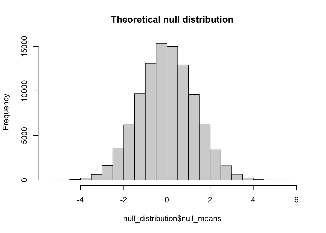
In discussion we made mention that due to the assumption of equal means and equal variances that the null distribution should approximate the form of the standard distribution were \(\mu=0\) and \(\sigma = 1\). This fact allows us to say something about the probability of an observed difference as a probability of obtaining a Z-score that far removed from 0.
17.9 Probabilty of observed differences
Continuing on from the previous section, we have our null distribution of IQ scores, appropriately named null_distribution. This is the theoretical distribution of differences assuming the two populations are the same. Simply put, this is the distribution of differences we might expect if our advanced curriculum did not have any impact. You’ll note that even assuming that the two groups are identical still yields some differences by chance:
max(null_distribution$null_means)[1] 5.514248min(null_distribution$null_means)[1] -5.409361but that the probability of those extremes is very, very low (but still exists which is why we never prove the alternative hypothesis). Let’s say I take a sample from pop_basic and pop_advanced and find that my means differ by 3. Given the null distribution, what is the probability that I will observe a difference this large? To derive this probability, we take advantage of what we know about the standard distribution, where we have a known probability of obtaining any given Z-score.
The process of answering the above is as follows: 1. transform the observed difference to a Z-score using the mean and SD of the null distribution; 2. calculate the probability of that extreme of a score.
Here is step 1:
# 1. convert the observed difference to a z-score:
Zscore <- (3-mean(null_distribution$null_means))/sd(null_distribution$null_means)
show(Zscore)
[1] 2.339173I want to pause here to note that the obtained Z-score is positive. As a result the score is on the right side of the distribution. Our probability function, pnorm() returns the probability of an obtained score or lower (the cumulative probability). However, we want the probability of the observed score or more extreme. In this case more extreme means greater than. Conversely if the observed Z score is less than 0, then more extreme means less than. I bring this up as this determines what value we use to calculate the desired probability. In the latter case, less than we can simple take the output of pnorm() and call it a day. However, in cases like ours, when \(Z>0\) we need to use 1-pnorm().
OK, on to the calculation:
Zscore <- (3-mean(null_distribution$null_means))/sd(null_distribution$null_means)
1-pnorm(Zscore)
[1] 0.009663249Based on a criteria of rejecting the null if \(p<.05\) we would reject here. BUT NOTE: not necessarily because it’s less than .05. Remember that if I have a two-tailed test, my criteria requires that I split my \(\alpha\). So in truth I need to obtain a value less than .025 in either direction.
17.10 A note about sample size
So I got a pretty low p-value, but you might say it was expected given that my sample size was 250 for each group. Let’s see what happens if I drop the sample size down to 10 students per group, creating a new null distribution, null_distribution_10:
# create an empty vector to store the null difference in means
null_distribution_10 <-
  tibble(simulation = 1:100000) %>%
  group_by(simulation) %>%
  mutate(control_sample1 = mean(sample(pop_basic,size = 10,replace = T)),
         control_sample2 = mean(sample(pop_basic, size = 10, replace = T)),
         null_means = control_sample1-control_sample2)
What does this distribution look like?
hist(null_distribution_10$null_means, main = "Theoretical null distribution")
mean(null_distribution_10$null_means)[1] 0.01041048And let’s take a look at the probability of an observed difference of 3 in this case. Not that I’m using the pnorm() shortcut so I don’t need to calculate my Z by hand:
1-pnorm(q = 3,mean = mean(null_distribution_10$null_means),sd = sd(null_distribution_10$null_means))[1] 0.3211936As we can see, size matters. Given that we are omnipotent in this case, we know the truth of the matter is that the two populations are in fact different, and that the mean of pop_basic is not equal to the mean of pop_advanced. Thus what we have here is a failure to reject the null hypothesis when it is indeed false. Hmm, what kind of error is that again? This last example is going to figure prominently in our discussions of power and what power is, properly defined. For now, I think this is a good place to stop this week.